Quantum Mechanics Note
Date: 2024/05/27Categories: Physics
Tags: Physics, Quantum Mechanics
Read Time: 12 minutes
0.1 Contents
- 0.2 Probability Basics
- 0.3 Calculus Basics
- 0.4 Wave Function
- 0.5 Schrödinger Equation
- 0.6 Double Slit Experiment
- 0.7 Parity of TISE Solutions
- 0.8 States of TISE Solutions
- 0.9 Continuity Equation and Probability Current
- 0.10 Quantum Tunnelling
- 0.11 Functional Analysis of Quantum Mechanics
- 0.12 Measurement Postulate
- 0.13 Measurement of Observables
- 0.14 Commutators and Lie Bracket
- 0.15 Compatibility of Observables
- 0.16 Robertson Inequality
- 0.17 Quantum Harmonic Oscillator
- 0.18 Constant of Motion and Commutators
0.2 Probability Basics
0.2.1 Random Variable
A random variable %22%2F%3E%3C%2Fg%3E%3C%2Fg%3E%3Cdefs%3E%3Csymbol%20id%3D%22a%22%20overflow%3D%22visible%22%3E%3Cpath%20d%3D%22M12.51%2010.245c-.255%200-1.14-.045-1.395-.045-.3%200-1.35.045-1.65.045-.225%200-.345-.12-.345-.36%200-.135.075-.21.24-.225.36-.045.54-.165.54-.39q0-.203-.27-.495l-2.34-2.52C6.855%207.275%206.435%208.28%206%209.3a.2.2%200%200%200%20.075.09c.135.15.39.24.75.27.24.03.36.15.36.345%200%20.165-.09.24-.285.24-.36%200-1.515-.045-1.875-.045-.315%200-1.35.045-1.665.045-.225%200-.33-.12-.33-.36q0-.225.405-.225c.675%200%20.885%200%201.065-.435L6.24%205.13%203.12%201.785a1%201%200%200%200-.18-.15C2.325.99%201.62.63.795.585.54.57.405.435.405.21.45.075.465%200%20.66%200%20.915%200%201.8.045%202.055.045%202.37.045%203.405%200%203.72%200c.225%200%20.33.12.33.36%200%20.135-.075.21-.24.225-.36.03-.54.165-.54.39%200%20.15.135.36.39.63.93.99%201.875%201.98%202.79%202.985.51-1.215%201.035-2.415%201.53-3.645-.015-.03-.03-.06-.075-.105C7.77.705%207.53.63%207.17.585c-.225-.03-.345-.15-.345-.345%200-.165.09-.24.285-.24l1.875.045C9.3.045%2010.35%200%2010.62%200c.225%200%20.345.12.345.345%200%20.15-.105.225-.33.24-.465%200-.765.015-.87.075S9.54.9%209.42%201.2L7.515%205.745c1.02%201.08%201.785%201.89%202.28%202.445.36.375.6.63.735.735.555.465%201.17.705%201.845.735.315.015.39.09.39.375-.045.135-.06.21-.255.21%22%2F%3E%3C%2Fsymbol%3E%3C%2Fdefs%3E%3C%2Fsvg%3E) is a function that maps the sample space
is a function that maps the sample space %22%2F%3E%3C%2Fg%3E%3C%2Fg%3E%3Cdefs%3E%3Csymbol%20id%3D%22a%22%20overflow%3D%22visible%22%3E%3Cpath%20d%3D%22M4.005.375c0%20.72-.27%201.83-.795%203.315-.495%201.335-.735%202.37-.735%203.12%200%201.83%201.14%203.315%202.925%203.315S8.34%208.64%208.34%206.81c0-.735-.285-1.89-.84-3.435-.465-1.32-.69-2.325-.69-3%200-.36.06-.375.435-.375H9.66l.51%202.52h-.495q-.135-.72-.27-1.125c-.06-.165-.195-.255-.39-.3-.045-.015-.225-.015-.54-.015h-1.11q.225.855%201.305%202.43%201.305%201.957%201.305%203.285c0%201.125-.495%202.055-1.47%202.79-.885.66-1.92.99-3.09.99q-1.777%200-3.105-.99c-.975-.72-1.47-1.65-1.47-2.79q0-1.305%201.305-3.285c.57-.84%201.065-1.575%201.305-2.43H2.34c-.51%200-.81.075-.885.21-.15.48-.255.885-.315%201.23H.645L1.155%200h2.43c.345%200%20.42.03.42.375%22%2F%3E%3C%2Fsymbol%3E%3C%2Fdefs%3E%3C%2Fsvg%3E) to the real number line
to the real number line %22%2F%3E%3C%2Fg%3E%3C%2Fg%3E%3Cdefs%3E%3Csymbol%20id%3D%22a%22%20overflow%3D%22visible%22%3E%3Cpath%20d%3D%22M1.56%208.85V1.425c0-.75-.075-.78-.855-.78C.39.645.24.54.24.33.24.06.465%200%20.81%200h4.05c.375%200%20.555.105.555.33%200%20.21-.165.315-.48.315-.78%200-.84.03-.84.78V4.65h.435l2.22-3.405c.375-.6.6-.945.66-1.035.09-.135.27-.21.54-.21h2.04c.375%200%20.555.105.555.33%200%20.165-.09.27-.27.3-.375.075-.9.6-1.59%201.56a53%2053%200%200%200-1.8%202.64q2.565.495%202.565%202.61c0%201.005-.45%201.755-1.35%202.22-.78.405-1.665.615-2.64.615H.81c-.375%200-.57-.105-.57-.33%200-.21.15-.315.465-.315.78%200%20.855-.03.855-.78m6.465.105c.525-.315.78-.825.78-1.515%200-1.035-.6-1.665-1.785-1.92.255.42.39%201.05.39%201.905s-.165%201.515-.48%202.01a4%204%200%200%200%201.095-.48M6.78%207.425q0-1.395-.495-1.755c-.33-.24-1.065-.375-2.19-.375v3.6c0%20.555.21.735.855.735%201.425%200%201.83-.705%201.83-2.205M6.195%204.74C7.44%202.76%208.415%201.395%209.15.645H7.875L5.28%204.665a1%201%200%200%200%20.18.015c.21%200%20.45.015.735.06M2.1%209.63h1.5c-.09-.165-.135-.39-.135-.69V1.395c0-.315.03-.57.09-.75H2.1c.06.18.09.435.09.75V8.88c0%20.315-.03.57-.09.75%22%2F%3E%3C%2Fsymbol%3E%3C%2Fdefs%3E%3C%2Fsvg%3E) .
.
0.2.2 Probability Density Function
The probability density function %22%2F%3E%3Cuse%20xlink%3Ahref%3D%22%23b%22%20class%3D%22typst-text%22%20transform%3D%22matrix(1%200%200%20-1%209.7%2012.22)%22%2F%3E%3Cuse%20xlink%3Ahref%3D%22%23c%22%20class%3D%22typst-text%22%20transform%3D%22matrix(1%200%200%20-1%2015.535%2012.22)%22%2F%3E%3Cuse%20xlink%3Ahref%3D%22%23d%22%20class%3D%22typst-text%22%20transform%3D%22matrix(1%200%200%20-1%2024.115%2012.22)%22%2F%3E%3C%2Fg%3E%3C%2Fg%3E%3Cdefs%3E%3Csymbol%20id%3D%22a%22%20overflow%3D%22visible%22%3E%3Cpath%20d%3D%22M8.28%209.495c0%20.66-.645%201.08-1.35%201.08-.93%200-1.575-.6-1.92-1.785-.075-.27-.24-1.035-.48-2.295h-.975c-.33%200-.495-.015-.495-.33%200-.165.15-.24.465-.24h.9L3.33.12c-.165-.855-.315-1.485-.45-1.905-.18-.555-.435-.84-.765-.84-.225%200-.405.06-.57.165.48.075.72.36.72.84%200%20.39-.195.585-.6.585-.51%200-.87-.45-.87-.96%200-.66.615-1.08%201.32-1.08.375%200%20.72.15%201.005.465.48.495.855%201.2%201.125%202.145.165.585.315%201.155.42%201.725l.87%204.665h1.23c.345%200%20.495.015.495.36%200%20.135-.15.21-.45.21H5.655c.09.615.51%202.88.645%203.165.15.315.36.465.63.465.225%200%20.42-.06.585-.165-.465-.105-.705-.375-.705-.84%200-.39.195-.585.6-.585.51%200%20.87.45.87.96%22%2F%3E%3C%2Fsymbol%3E%3Csymbol%20id%3D%22b%22%20overflow%3D%22visible%22%3E%3Cpath%20d%3D%22M4.77-3.72c.135%200%20.21.075.21.21%200%20.045-.03.105-.075.165-.78.6-1.41%201.59-1.875%202.955-.405%201.185-.615%202.355-.615%203.51v1.26c0%201.155.21%202.325.615%203.51.465%201.365%201.095%202.355%201.875%202.955a.24.24%200%200%201%20.075.165c0%20.135-.075.21-.21.21a.3.3%200%200%201-.105-.045c-.9-.69-1.65-1.71-2.265-3.075-.585-1.305-.885-2.535-.885-3.72V3.12c0-1.185.3-2.415.885-3.72.615-1.365%201.365-2.385%202.265-3.075a.3.3%200%200%201%20.105-.045%22%2F%3E%3C%2Fsymbol%3E%3Csymbol%20id%3D%22c%22%20overflow%3D%22visible%22%3E%3Cpath%20d%3D%22M7.905%205.595c0%20.69-.675%201.035-1.425%201.035-.645%200-1.155-.345-1.545-1.035-.315.69-.84%201.035-1.605%201.035-.735%200-1.335-.345-1.815-1.02C1.11%205.025.9%204.59.9%204.305c0-.135.075-.21.225-.21.135%200%20.225.075.255.21.285.87.915%201.89%201.92%201.89.495%200%20.735-.315.735-.93%200-.315-.27-1.485-.795-3.495C2.985.765%202.535.27%201.89.27c-.21%200-.405.045-.57.12q.585.225.585.81c0%20.39-.195.585-.6.585-.495%200-.87-.42-.87-.915%200-.69.705-1.035%201.44-1.035.63%200%201.14.345%201.545%201.035.285-.69.825-1.035%201.605-1.035.72%200%201.32.345%201.8%201.02.405.585.615%201.02.615%201.305%200%20.135-.075.21-.225.21-.135%200-.21-.075-.255-.21C6.705%201.305%206.03.27%205.055.27c-.495%200-.75.3-.75.915%200%20.195.075.615.24%201.29l.51%202.025c.285%201.125.75%201.695%201.41%201.695.21%200%20.405-.045.57-.12-.405-.135-.6-.405-.6-.81%200-.39.21-.585.615-.585.48%200%20.855.435.855.915%22%2F%3E%3C%2Fsymbol%3E%3Csymbol%20id%3D%22d%22%20overflow%3D%22visible%22%3E%3Cpath%20d%3D%22M1.17-3.675c.9.69%201.65%201.71%202.265%203.075.585%201.305.885%202.535.885%203.72v1.26c0%201.185-.3%202.415-.885%203.72-.615%201.365-1.365%202.385-2.265%203.075a.3.3%200%200%201-.105.045c-.135%200-.21-.075-.21-.21%200-.06.03-.12.075-.165.78-.6%201.41-1.59%201.875-2.955.405-1.185.615-2.355.615-3.51V3.12c0-1.155-.21-2.325-.615-3.51C2.34-1.755%201.71-2.745.93-3.345c-.045-.06-.075-.12-.075-.165%200-.135.075-.21.21-.21.015%200%20.06.015.105.045%22%2F%3E%3C%2Fsymbol%3E%3C%2Fdefs%3E%3C%2Fsvg%3E) of a random variable is a function that describes the likelihood of the random variable to take on a specific value.
of a random variable is a function that describes the likelihood of the random variable to take on a specific value.
0.2.3 Cumulative Distribution Function
The cumulative distribution function %22%2F%3E%3Cuse%20xlink%3Ahref%3D%22%23b%22%20class%3D%22typst-text%22%20transform%3D%22matrix(1%200%200%20-1%2012.655%2012.22)%22%2F%3E%3Cuse%20xlink%3Ahref%3D%22%23c%22%20class%3D%22typst-text%22%20transform%3D%22matrix(1%200%200%20-1%2018.49%2012.22)%22%2F%3E%3Cuse%20xlink%3Ahref%3D%22%23d%22%20class%3D%22typst-text%22%20transform%3D%22matrix(1%200%200%20-1%2027.07%2012.22)%22%2F%3E%3C%2Fg%3E%3C%2Fg%3E%3Cdefs%3E%3Csymbol%20id%3D%22a%22%20overflow%3D%22visible%22%3E%3Cpath%20d%3D%22M2.985%209.84c0-.15.165-.225.48-.225.6%200%20.9-.06.9-.195%200-.045-.03-.15-.075-.345L2.34%201.23C2.25.9%202.1.705%201.89.63%201.785.6%201.515.585%201.05.585.72.585.57.555.57.24.57.075.66%200%20.855%200l1.95.045L5.025%200c.24%200%20.36.12.36.345%200%20.255-.165.24-.555.24-.66%200-1.035.03-1.125.105-.045.015-.06.075-.06.15l.96%203.975H6c.69%200%201.17-.03%201.17-.6%200-.195-.03-.435-.105-.72a3%203%200%200%201-.045-.165c0-.165.075-.24.24-.24.075.015.18.12.285.345l.81%203.225c.03.12.045.21.045.255-.045.135-.135.21-.24.21-.12%200-.21-.12-.27-.345-.15-.57-.36-.93-.6-1.11q-.36-.27-1.26-.27H4.755l.93%203.69c.12.51.12.525.75.525h1.95c1.455%200%202.115-.225%202.115-1.56%200-.3-.015-.57-.045-.795-.015-.165-.03-.255-.03-.27%200-.165.075-.24.225-.24s.24.135.27.42l.3%202.565c.045.42-.06.465-.465.465h-7.26c-.345%200-.51-.015-.51-.36%22%2F%3E%3C%2Fsymbol%3E%3Csymbol%20id%3D%22b%22%20overflow%3D%22visible%22%3E%3Cpath%20d%3D%22M4.77-3.72c.135%200%20.21.075.21.21%200%20.045-.03.105-.075.165-.78.6-1.41%201.59-1.875%202.955-.405%201.185-.615%202.355-.615%203.51v1.26c0%201.155.21%202.325.615%203.51.465%201.365%201.095%202.355%201.875%202.955a.24.24%200%200%201%20.075.165c0%20.135-.075.21-.21.21a.3.3%200%200%201-.105-.045c-.9-.69-1.65-1.71-2.265-3.075-.585-1.305-.885-2.535-.885-3.72V3.12c0-1.185.3-2.415.885-3.72.615-1.365%201.365-2.385%202.265-3.075a.3.3%200%200%201%20.105-.045%22%2F%3E%3C%2Fsymbol%3E%3Csymbol%20id%3D%22c%22%20overflow%3D%22visible%22%3E%3Cpath%20d%3D%22M7.905%205.595c0%20.69-.675%201.035-1.425%201.035-.645%200-1.155-.345-1.545-1.035-.315.69-.84%201.035-1.605%201.035-.735%200-1.335-.345-1.815-1.02C1.11%205.025.9%204.59.9%204.305c0-.135.075-.21.225-.21.135%200%20.225.075.255.21.285.87.915%201.89%201.92%201.89.495%200%20.735-.315.735-.93%200-.315-.27-1.485-.795-3.495C2.985.765%202.535.27%201.89.27c-.21%200-.405.045-.57.12q.585.225.585.81c0%20.39-.195.585-.6.585-.495%200-.87-.42-.87-.915%200-.69.705-1.035%201.44-1.035.63%200%201.14.345%201.545%201.035.285-.69.825-1.035%201.605-1.035.72%200%201.32.345%201.8%201.02.405.585.615%201.02.615%201.305%200%20.135-.075.21-.225.21-.135%200-.21-.075-.255-.21C6.705%201.305%206.03.27%205.055.27c-.495%200-.75.3-.75.915%200%20.195.075.615.24%201.29l.51%202.025c.285%201.125.75%201.695%201.41%201.695.21%200%20.405-.045.57-.12-.405-.135-.6-.405-.6-.81%200-.39.21-.585.615-.585.48%200%20.855.435.855.915%22%2F%3E%3C%2Fsymbol%3E%3Csymbol%20id%3D%22d%22%20overflow%3D%22visible%22%3E%3Cpath%20d%3D%22M1.17-3.675c.9.69%201.65%201.71%202.265%203.075.585%201.305.885%202.535.885%203.72v1.26c0%201.185-.3%202.415-.885%203.72-.615%201.365-1.365%202.385-2.265%203.075a.3.3%200%200%201-.105.045c-.135%200-.21-.075-.21-.21%200-.06.03-.12.075-.165.78-.6%201.41-1.59%201.875-2.955.405-1.185.615-2.355.615-3.51V3.12c0-1.155-.21-2.325-.615-3.51C2.34-1.755%201.71-2.745.93-3.345c-.045-.06-.075-.12-.075-.165%200-.135.075-.21.21-.21.015%200%20.06.015.105.045%22%2F%3E%3C%2Fsymbol%3E%3C%2Fdefs%3E%3C%2Fsvg%3E) of a random variable is a function that describes the probability that the random variable takes on a value less than or equal to
of a random variable is a function that describes the probability that the random variable takes on a value less than or equal to %22%2F%3E%3C%2Fg%3E%3C%2Fg%3E%3Cdefs%3E%3Csymbol%20id%3D%22a%22%20overflow%3D%22visible%22%3E%3Cpath%20d%3D%22M7.905%205.595c0%20.69-.675%201.035-1.425%201.035-.645%200-1.155-.345-1.545-1.035-.315.69-.84%201.035-1.605%201.035-.735%200-1.335-.345-1.815-1.02C1.11%205.025.9%204.59.9%204.305c0-.135.075-.21.225-.21.135%200%20.225.075.255.21.285.87.915%201.89%201.92%201.89.495%200%20.735-.315.735-.93%200-.315-.27-1.485-.795-3.495C2.985.765%202.535.27%201.89.27c-.21%200-.405.045-.57.12q.585.225.585.81c0%20.39-.195.585-.6.585-.495%200-.87-.42-.87-.915%200-.69.705-1.035%201.44-1.035.63%200%201.14.345%201.545%201.035.285-.69.825-1.035%201.605-1.035.72%200%201.32.345%201.8%201.02.405.585.615%201.02.615%201.305%200%20.135-.075.21-.225.21-.135%200-.21-.075-.255-.21C6.705%201.305%206.03.27%205.055.27c-.495%200-.75.3-.75.915%200%20.195.075.615.24%201.29l.51%202.025c.285%201.125.75%201.695%201.41%201.695.21%200%20.405-.045.57-.12-.405-.135-.6-.405-.6-.81%200-.39.21-.585.615-.585.48%200%20.855.435.855.915%22%2F%3E%3C%2Fsymbol%3E%3C%2Fdefs%3E%3C%2Fsvg%3E) .
.

0.2.4 Expectation
The expectation of a random variable is the average value of the random variable.

0.2.5 Variance
The variance of a random variable is a measure of how much the values of the random variable vary.
%22%2F%3E%3Cuse%20xlink%3Ahref%3D%22%23b%22%20class%3D%22typst-text%22%20transform%3D%22matrix(1%200%200%20-1%2022.495%2028.177)%22%2F%3E%3Cuse%20xlink%3Ahref%3D%22%23c%22%20class%3D%22typst-text%22%20transform%3D%22matrix(1%200%200%20-1%2035.68%2022.732)%22%2F%3E%3Cuse%20xlink%3Ahref%3D%22%23d%22%20class%3D%22typst-text%22%20transform%3D%22matrix(1%200%200%20-1%2046.661%2028.177)%22%2F%3E%3Cuse%20xlink%3Ahref%3D%22%23e%22%20class%3D%22typst-text%22%20transform%3D%22matrix(1%200%200%20-1%2058.331%2028.177)%22%2F%3E%3Cuse%20xlink%3Ahref%3D%22%23f%22%20class%3D%22typst-text%22%20transform%3D%22matrix(1%200%200%20-1%2074.168%2028.177)%22%2F%3E%3Cuse%20xlink%3Ahref%3D%22%23b%22%20class%3D%22typst-text%22%20transform%3D%22matrix(1%200%200%20-1%2080.003%2028.177)%22%2F%3E%3Cuse%20xlink%3Ahref%3D%22%23g%22%20class%3D%22typst-text%22%20transform%3D%22matrix(1%200%200%20-1%2096.521%2028.177)%22%2F%3E%3Cuse%20xlink%3Ahref%3D%22%23e%22%20class%3D%22typst-text%22%20transform%3D%22matrix(1%200%200%20-1%20112.358%2028.177)%22%2F%3E%3Cuse%20xlink%3Ahref%3D%22%23b%22%20class%3D%22typst-text%22%20transform%3D%22matrix(1%200%200%20-1%20128.195%2028.177)%22%2F%3E%3Cuse%20xlink%3Ahref%3D%22%23h%22%20class%3D%22typst-text%22%20transform%3D%22matrix(1%200%200%20-1%20145.546%2028.177)%22%2F%3E%3Cuse%20xlink%3Ahref%3D%22%23i%22%20class%3D%22typst-text%22%20transform%3D%22matrix(1%200%200%20-1%20157.216%2028.177)%22%2F%3E%3Cuse%20xlink%3Ahref%3D%22%23c%22%20class%3D%22typst-text%22%20transform%3D%22matrix(1%200%200%20-1%20163.051%2022.732)%22%2F%3E%3Cuse%20xlink%3Ahref%3D%22%23h%22%20class%3D%22typst-text%22%20transform%3D%22matrix(1%200%200%20-1%20174.032%2028.177)%22%2F%3E%3Cuse%20xlink%3Ahref%3D%22%23d%22%20class%3D%22typst-text%22%20transform%3D%22matrix(1%200%200%20-1%20185.702%2028.177)%22%2F%3E%3Cuse%20xlink%3Ahref%3D%22%23e%22%20class%3D%22typst-text%22%20transform%3D%22matrix(1%200%200%20-1%20197.372%2028.177)%22%2F%3E%3Cuse%20xlink%3Ahref%3D%22%23b%22%20class%3D%22typst-text%22%20transform%3D%22matrix(1%200%200%20-1%20213.209%2028.177)%22%2F%3E%3Cuse%20xlink%3Ahref%3D%22%23c%22%20class%3D%22typst-text%22%20transform%3D%22matrix(1%200%200%20-1%20226.394%2022.732)%22%2F%3E%3Cuse%20xlink%3Ahref%3D%22%23h%22%20class%3D%22typst-text%22%20transform%3D%22matrix(1%200%200%20-1%20237.375%2028.177)%22%2F%3E%3Cuse%20xlink%3Ahref%3D%22%23g%22%20class%3D%22typst-text%22%20transform%3D%22matrix(1%200%200%20-1%20253.212%2028.177)%22%2F%3E%3Cuse%20xlink%3Ahref%3D%22%23e%22%20class%3D%22typst-text%22%20transform%3D%22matrix(1%200%200%20-1%20269.049%2028.177)%22%2F%3E%3Cuse%20xlink%3Ahref%3D%22%23b%22%20class%3D%22typst-text%22%20transform%3D%22matrix(1%200%200%20-1%20284.885%2028.177)%22%2F%3E%3Cuse%20xlink%3Ahref%3D%22%23h%22%20class%3D%22typst-text%22%20transform%3D%22matrix(1%200%200%20-1%20302.237%2028.177)%22%2F%3E%3Cuse%20xlink%3Ahref%3D%22%23c%22%20class%3D%22typst-text%22%20transform%3D%22matrix(1%200%200%20-1%20305.085%2016.972)%22%2F%3E%3Cuse%20xlink%3Ahref%3D%22%23j%22%20class%3D%22typst-text%22%20transform%3D%22matrix(1%200%200%20-1%20318.074%2028.177)%22%2F%3E%3C%2Fg%3E%3C%2Fg%3E%3Cdefs%3E%3Csymbol%20id%3D%22a%22%20overflow%3D%22visible%22%3E%3Cpath%20d%3D%22M11.385%200c.255%200%20.39.06.39.195l-5.1%2010.245c-.105.195-.24.3-.435.3s-.33-.105-.435-.3L.78.375C.735.27.705.21.705.18c0-.12.135-.18.39-.18ZM5.76%209.06l3.9-7.815h-7.8Z%22%2F%3E%3C%2Fsymbol%3E%3Csymbol%20id%3D%22b%22%20overflow%3D%22visible%22%3E%3Cpath%20d%3D%22M12.51%2010.245c-.255%200-1.14-.045-1.395-.045-.3%200-1.35.045-1.65.045-.225%200-.345-.12-.345-.36%200-.135.075-.21.24-.225.36-.045.54-.165.54-.39q0-.203-.27-.495l-2.34-2.52C6.855%207.275%206.435%208.28%206%209.3a.2.2%200%200%200%20.075.09c.135.15.39.24.75.27.24.03.36.15.36.345%200%20.165-.09.24-.285.24-.36%200-1.515-.045-1.875-.045-.315%200-1.35.045-1.665.045-.225%200-.33-.12-.33-.36q0-.225.405-.225c.675%200%20.885%200%201.065-.435L6.24%205.13%203.12%201.785a1%201%200%200%200-.18-.15C2.325.99%201.62.63.795.585.54.57.405.435.405.21.45.075.465%200%20.66%200%20.915%200%201.8.045%202.055.045%202.37.045%203.405%200%203.72%200c.225%200%20.33.12.33.36%200%20.135-.075.21-.24.225-.36.03-.54.165-.54.39%200%20.15.135.36.39.63.93.99%201.875%201.98%202.79%202.985.51-1.215%201.035-2.415%201.53-3.645-.015-.03-.03-.06-.075-.105C7.77.705%207.53.63%207.17.585c-.225-.03-.345-.15-.345-.345%200-.165.09-.24.285-.24l1.875.045C9.3.045%2010.35%200%2010.62%200c.225%200%20.345.12.345.345%200%20.15-.105.225-.33.24-.465%200-.765.015-.87.075S9.54.9%209.42%201.2L7.515%205.745c1.02%201.08%201.785%201.89%202.28%202.445.36.375.6.63.735.735.555.465%201.17.705%201.845.735.315.015.39.09.39.375-.045.135-.06.21-.255.21%22%2F%3E%3C%2Fsymbol%3E%3Csymbol%20id%3D%22c%22%20overflow%3D%22visible%22%3E%3Cpath%20d%3D%22M1.25%204.452c.335%200%20.587.252.587.588%200%20.378-.199.577-.587.588.23.494.756.892%201.438.892.924%200%201.533-.692%201.533-1.616%200-.505-.178-.988-.546-1.46a5%205%200%200%200-.41-.504L.777.473C.64.347.661.315.661%200h4.326l.326%201.974h-.441c-.074-.556-.157-.882-.252-.955-.053-.032-.378-.053-.997-.053H1.837c.704.62%201.355%201.176%201.974%201.67.473.367.809.692%201.019.976q.473.614.473%201.292c0%20.65-.252%201.165-.767%201.543-.451.346-1.018.525-1.69.525a2.36%202.36%200%200%201-1.502-.504c-.452-.367-.683-.83-.683-1.396%200-.357.263-.62.589-.62%22%2F%3E%3C%2Fsymbol%3E%3Csymbol%20id%3D%22d%22%20overflow%3D%22visible%22%3E%3Cpath%20d%3D%22M10.47%205.505H1.2c-.24%200-.36-.12-.36-.345s.12-.345.36-.345h9.27c.24%200%20.36.12.36.345%200%20.18-.165.345-.36.345m0-2.82H1.2c-.24%200-.36-.12-.36-.345s.12-.345.36-.345h9.27c.24%200%20.36.12.36.345a.35.35%200%200%201-.36.345%22%2F%3E%3C%2Fsymbol%3E%3Csymbol%20id%3D%22e%22%20overflow%3D%22visible%22%3E%3Cpath%20d%3D%22M9.99-.675c.255-.105.525.09.525.33%200%20.15-.075.255-.21.315l-8.01%203.78%208.01%203.78c.135.06.21.165.21.3%200%20.255-.12.375-.36.375a.5.5%200%200%201-.165-.03l-8.61-4.08c-.15-.075-.225-.18-.225-.345s.075-.27.225-.345Z%22%2F%3E%3C%2Fsymbol%3E%3Csymbol%20id%3D%22f%22%20overflow%3D%22visible%22%3E%3Cpath%20d%3D%22M4.77-3.72c.135%200%20.21.075.21.21%200%20.045-.03.105-.075.165-.78.6-1.41%201.59-1.875%202.955-.405%201.185-.615%202.355-.615%203.51v1.26c0%201.155.21%202.325.615%203.51.465%201.365%201.095%202.355%201.875%202.955a.24.24%200%200%201%20.075.165c0%20.135-.075.21-.21.21a.3.3%200%200%201-.105-.045c-.9-.69-1.65-1.71-2.265-3.075-.585-1.305-.885-2.535-.885-3.72V3.12c0-1.185.3-2.415.885-3.72.615-1.365%201.365-2.385%202.265-3.075a.3.3%200%200%201%20.105-.045%22%2F%3E%3C%2Fsymbol%3E%3Csymbol%20id%3D%22g%22%20overflow%3D%22visible%22%3E%3Cpath%20d%3D%22M10.47%204.05H1.2c-.24%200-.36-.105-.36-.3s.12-.3.36-.3h9.27c.24%200%20.36.105.36.3%200%20.18-.18.3-.36.3%22%2F%3E%3C%2Fsymbol%3E%3Csymbol%20id%3D%22h%22%20overflow%3D%22visible%22%3E%3Cpath%20d%3D%22M10.29%203.405c.15.075.225.18.225.345s-.075.27-.225.345l-8.61%204.08a.5.5%200%200%201-.165.03c-.24%200-.36-.12-.36-.375%200-.135.075-.24.21-.3l8.01-3.78-8.01-3.78c-.135-.06-.21-.165-.21-.3%200-.255.12-.375.36-.375.06%200%20.12.015.165.03Z%22%2F%3E%3C%2Fsymbol%3E%3Csymbol%20id%3D%22i%22%20overflow%3D%22visible%22%3E%3Cpath%20d%3D%22M1.17-3.675c.9.69%201.65%201.71%202.265%203.075.585%201.305.885%202.535.885%203.72v1.26c0%201.185-.3%202.415-.885%203.72-.615%201.365-1.365%202.385-2.265%203.075a.3.3%200%200%201-.105.045c-.135%200-.21-.075-.21-.21%200-.06.03-.12.075-.165.78-.6%201.41-1.59%201.875-2.955.405-1.185.615-2.355.615-3.51V3.12c0-1.155-.21-2.325-.615-3.51C2.34-1.755%201.71-2.745.93-3.345c-.045-.06-.075-.12-.075-.165%200-.135.075-.21.21-.21.015%200%20.06.015.105.045%22%2F%3E%3C%2Fsymbol%3E%3Csymbol%20id%3D%22j%22%20overflow%3D%22visible%22%3E%3Cpath%20d%3D%22M2.88.795a.8.8%200%200%201-.795.795.8.8%200%200%201-.795-.795A.8.8%200%200%201%202.085%200a.8.8%200%200%201%20.795.795%22%2F%3E%3C%2Fsymbol%3E%3C%2Fdefs%3E%3C%2Fsvg%3E)
0.2.6 Standard Deviation
The standard deviation of a random variable is the square root of the variance.
%22%2F%3E%3Cuse%20xlink%3Ahref%3D%22%23b%22%20class%3D%22typst-text%22%20transform%3D%22matrix(1%200%200%20-1%2022.495%2025.343)%22%2F%3E%3Cuse%20xlink%3Ahref%3D%22%23c%22%20class%3D%22typst-text%22%20transform%3D%22matrix(1%200%200%20-1%2039.847%2025.343)%22%2F%3E%3Cuse%20xlink%3Ahref%3D%22%23d%22%20class%3D%22typst-text%22%20transform%3D%22matrix(1%200%200%20-1%2055.683%2011.32)%22%2F%3E%3Cpath%20fill%3D%22none%22%20stroke%3D%22%23000%22%20stroke-width%3D%22.72%22%20d%3D%22M68.178%2011.08h32.495%22%20class%3D%22typst-shape%22%2F%3E%3Cuse%20xlink%3Ahref%3D%22%23a%22%20class%3D%22typst-text%22%20transform%3D%22matrix(1%200%200%20-1%2068.178%2025.343)%22%2F%3E%3Cuse%20xlink%3Ahref%3D%22%23b%22%20class%3D%22typst-text%22%20transform%3D%22matrix(1%200%200%20-1%2080.673%2025.343)%22%2F%3E%3Cuse%20xlink%3Ahref%3D%22%23e%22%20class%3D%22typst-text%22%20transform%3D%22matrix(1%200%200%20-1%2093.858%2021.009)%22%2F%3E%3Cuse%20xlink%3Ahref%3D%22%23f%22%20class%3D%22typst-text%22%20transform%3D%22matrix(1%200%200%20-1%20100.673%2025.343)%22%2F%3E%3C%2Fg%3E%3C%2Fg%3E%3Cdefs%3E%3Csymbol%20id%3D%22a%22%20overflow%3D%22visible%22%3E%3Cpath%20d%3D%22M11.385%200c.255%200%20.39.06.39.195l-5.1%2010.245c-.105.195-.24.3-.435.3s-.33-.105-.435-.3L.78.375C.735.27.705.21.705.18c0-.12.135-.18.39-.18ZM5.76%209.06l3.9-7.815h-7.8Z%22%2F%3E%3C%2Fsymbol%3E%3Csymbol%20id%3D%22b%22%20overflow%3D%22visible%22%3E%3Cpath%20d%3D%22M12.51%2010.245c-.255%200-1.14-.045-1.395-.045-.3%200-1.35.045-1.65.045-.225%200-.345-.12-.345-.36%200-.135.075-.21.24-.225.36-.045.54-.165.54-.39q0-.203-.27-.495l-2.34-2.52C6.855%207.275%206.435%208.28%206%209.3a.2.2%200%200%200%20.075.09c.135.15.39.24.75.27.24.03.36.15.36.345%200%20.165-.09.24-.285.24-.36%200-1.515-.045-1.875-.045-.315%200-1.35.045-1.665.045-.225%200-.33-.12-.33-.36q0-.225.405-.225c.675%200%20.885%200%201.065-.435L6.24%205.13%203.12%201.785a1%201%200%200%200-.18-.15C2.325.99%201.62.63.795.585.54.57.405.435.405.21.45.075.465%200%20.66%200%20.915%200%201.8.045%202.055.045%202.37.045%203.405%200%203.72%200c.225%200%20.33.12.33.36%200%20.135-.075.21-.24.225-.36.03-.54.165-.54.39%200%20.15.135.36.39.63.93.99%201.875%201.98%202.79%202.985.51-1.215%201.035-2.415%201.53-3.645-.015-.03-.03-.06-.075-.105C7.77.705%207.53.63%207.17.585c-.225-.03-.345-.15-.345-.345%200-.165.09-.24.285-.24l1.875.045C9.3.045%2010.35%200%2010.62%200c.225%200%20.345.12.345.345%200%20.15-.105.225-.33.24-.465%200-.765.015-.87.075S9.54.9%209.42%201.2L7.515%205.745c1.02%201.08%201.785%201.89%202.28%202.445.36.375.6.63.735.735.555.465%201.17.705%201.845.735.315.015.39.09.39.375-.045.135-.06.21-.255.21%22%2F%3E%3C%2Fsymbol%3E%3Csymbol%20id%3D%22c%22%20overflow%3D%22visible%22%3E%3Cpath%20d%3D%22M10.47%205.505H1.2c-.24%200-.36-.12-.36-.345s.12-.345.36-.345h9.27c.24%200%20.36.12.36.345%200%20.18-.165.345-.36.345m0-2.82H1.2c-.24%200-.36-.12-.36-.345s.12-.345.36-.345h9.27c.24%200%20.36.12.36.345a.35.35%200%200%201-.36.345%22%2F%3E%3C%2Fsymbol%3E%3Csymbol%20id%3D%22d%22%20overflow%3D%22visible%22%3E%3Cpath%20d%3D%22M12.705-.03q.09.203.09.27%200%20.36-.36.36a.31.31%200%200%201-.3-.195c-2.145-4.29-3.21-6.45-3.21-6.48v-.015c0-.105-1.02-2.28-3.075-6.555l-2.595%205.73c-.075.165-.15.24-.24.24-.045%200-.135-.045-.255-.135L1.29-7.92c-.135-.105-.195-.18-.195-.255%200-.15.075-.225.21-.225.045%200%20.12.045.24.135l.72.525%202.91-6.405c.075-.165.18-.255.33-.255.18%200%20.3.075.375.21Z%22%2F%3E%3C%2Fsymbol%3E%3Csymbol%20id%3D%22e%22%20overflow%3D%22visible%22%3E%3Cpath%20d%3D%22M1.25%204.452c.335%200%20.587.252.587.588%200%20.378-.199.577-.587.588.23.494.756.892%201.438.892.924%200%201.533-.692%201.533-1.616%200-.505-.178-.988-.546-1.46a5%205%200%200%200-.41-.504L.777.473C.64.347.661.315.661%200h4.326l.326%201.974h-.441c-.074-.556-.157-.882-.252-.955-.053-.032-.378-.053-.997-.053H1.837c.704.62%201.355%201.176%201.974%201.67.473.367.809.692%201.019.976q.473.614.473%201.292c0%20.65-.252%201.165-.767%201.543-.451.346-1.018.525-1.69.525a2.36%202.36%200%200%201-1.502-.504c-.452-.367-.683-.83-.683-1.396%200-.357.263-.62.589-.62%22%2F%3E%3C%2Fsymbol%3E%3Csymbol%20id%3D%22f%22%20overflow%3D%22visible%22%3E%3Cpath%20d%3D%22M2.88.795a.8.8%200%200%201-.795.795.8.8%200%200%201-.795-.795A.8.8%200%200%201%202.085%200a.8.8%200%200%201%20.795.795%22%2F%3E%3C%2Fsymbol%3E%3C%2Fdefs%3E%3C%2Fsvg%3E)
0.2.7 Probability Amplitude
The probability amplitude %22%2F%3E%3Cuse%20xlink%3Ahref%3D%22%23b%22%20class%3D%22typst-text%22%20transform%3D%22matrix(1%200%200%20-1%2010.945%2012.22)%22%2F%3E%3Cuse%20xlink%3Ahref%3D%22%23c%22%20class%3D%22typst-text%22%20transform%3D%22matrix(1%200%200%20-1%2016.78%2012.22)%22%2F%3E%3Cuse%20xlink%3Ahref%3D%22%23d%22%20class%3D%22typst-text%22%20transform%3D%22matrix(1%200%200%20-1%2025.36%2012.22)%22%2F%3E%3C%2Fg%3E%3C%2Fg%3E%3Cdefs%3E%3Csymbol%20id%3D%22a%22%20overflow%3D%22visible%22%3E%3Cpath%20d%3D%22M8.01%205.895c0-.135.075-.285.24-.45.345-.33.525-.735.525-1.215%200-.435-.135-.9-.42-1.425C7.83%201.8%207.14%201.08%206.315.645A3.4%203.4%200%200%200%204.83.255l2.43%209.69c.03.135.045.21.045.24%200%20.15-.075.225-.24.225a.27.27%200%200%201-.165-.045c-.06-.12-.09-.225-.105-.3L4.35.285C3.285.42%202.76.96%202.76%201.89c0%20.405.27%201.32.795%202.745.105.3.165.555.165.75%200%20.75-.525%201.275-1.275%201.275-.675%200-1.185-.375-1.56-1.125q-.45-.9-.45-1.215c0-.135.075-.21.24-.21.195%200%20.225.09.285.3q.518%201.8%201.44%201.8.315%200%20.315-.405c0-.24-.105-.66-.33-1.26-.48-1.275-.72-2.115-.72-2.535q0-1.957%202.565-2.16c-.12-.525-.225-.96-.315-1.29-.225-.855-.345-1.335-.345-1.44.045-.12.06-.195.255-.195l.15.06c.09.24.165.465.21.66l.54%202.16q1.845.022%203.24%201.62a5.6%205.6%200%200%201%201.095%201.8c.315.825.465%201.605.465%202.34S9.285%206.66%208.82%206.66c-.39%200-.81-.375-.81-.765%22%2F%3E%3C%2Fsymbol%3E%3Csymbol%20id%3D%22b%22%20overflow%3D%22visible%22%3E%3Cpath%20d%3D%22M4.77-3.72c.135%200%20.21.075.21.21%200%20.045-.03.105-.075.165-.78.6-1.41%201.59-1.875%202.955-.405%201.185-.615%202.355-.615%203.51v1.26c0%201.155.21%202.325.615%203.51.465%201.365%201.095%202.355%201.875%202.955a.24.24%200%200%201%20.075.165c0%20.135-.075.21-.21.21a.3.3%200%200%201-.105-.045c-.9-.69-1.65-1.71-2.265-3.075-.585-1.305-.885-2.535-.885-3.72V3.12c0-1.185.3-2.415.885-3.72.615-1.365%201.365-2.385%202.265-3.075a.3.3%200%200%201%20.105-.045%22%2F%3E%3C%2Fsymbol%3E%3Csymbol%20id%3D%22c%22%20overflow%3D%22visible%22%3E%3Cpath%20d%3D%22M7.905%205.595c0%20.69-.675%201.035-1.425%201.035-.645%200-1.155-.345-1.545-1.035-.315.69-.84%201.035-1.605%201.035-.735%200-1.335-.345-1.815-1.02C1.11%205.025.9%204.59.9%204.305c0-.135.075-.21.225-.21.135%200%20.225.075.255.21.285.87.915%201.89%201.92%201.89.495%200%20.735-.315.735-.93%200-.315-.27-1.485-.795-3.495C2.985.765%202.535.27%201.89.27c-.21%200-.405.045-.57.12q.585.225.585.81c0%20.39-.195.585-.6.585-.495%200-.87-.42-.87-.915%200-.69.705-1.035%201.44-1.035.63%200%201.14.345%201.545%201.035.285-.69.825-1.035%201.605-1.035.72%200%201.32.345%201.8%201.02.405.585.615%201.02.615%201.305%200%20.135-.075.21-.225.21-.135%200-.21-.075-.255-.21C6.705%201.305%206.03.27%205.055.27c-.495%200-.75.3-.75.915%200%20.195.075.615.24%201.29l.51%202.025c.285%201.125.75%201.695%201.41%201.695.21%200%20.405-.045.57-.12-.405-.135-.6-.405-.6-.81%200-.39.21-.585.615-.585.48%200%20.855.435.855.915%22%2F%3E%3C%2Fsymbol%3E%3Csymbol%20id%3D%22d%22%20overflow%3D%22visible%22%3E%3Cpath%20d%3D%22M1.17-3.675c.9.69%201.65%201.71%202.265%203.075.585%201.305.885%202.535.885%203.72v1.26c0%201.185-.3%202.415-.885%203.72-.615%201.365-1.365%202.385-2.265%203.075a.3.3%200%200%201-.105.045c-.135%200-.21-.075-.21-.21%200-.06.03-.12.075-.165.78-.6%201.41-1.59%201.875-2.955.405-1.185.615-2.355.615-3.51V3.12c0-1.155-.21-2.325-.615-3.51C2.34-1.755%201.71-2.745.93-3.345c-.045-.06-.075-.12-.075-.165%200-.135.075-.21.21-.21.015%200%20.06.015.105.045%22%2F%3E%3C%2Fsymbol%3E%3C%2Fdefs%3E%3C%2Fsvg%3E) of a random variable is a complex value function that the likelihood of the random variable to take on value is given by
of a random variable is a complex value function that the likelihood of the random variable to take on value is given by %22%2F%3E%3Cuse%20xlink%3Ahref%3D%22%23b%22%20class%3D%22typst-text%22%20transform%3D%22matrix(1%200%200%20-1%2010.15%2013.417)%22%2F%3E%3Cuse%20xlink%3Ahref%3D%22%23c%22%20class%3D%22typst-text%22%20transform%3D%22matrix(1%200%200%20-1%2020.095%2013.417)%22%2F%3E%3Cuse%20xlink%3Ahref%3D%22%23d%22%20class%3D%22typst-text%22%20transform%3D%22matrix(1%200%200%20-1%2025.93%2013.417)%22%2F%3E%3Cuse%20xlink%3Ahref%3D%22%23e%22%20class%3D%22typst-text%22%20transform%3D%22matrix(1%200%200%20-1%2034.51%2013.417)%22%2F%3E%3Cuse%20xlink%3Ahref%3D%22%23a%22%20class%3D%22typst-text%22%20transform%3D%22matrix(1%200%200%20-1%2040.345%2013.417)%22%2F%3E%3Cuse%20xlink%3Ahref%3D%22%23f%22%20class%3D%22typst-text%22%20transform%3D%22matrix(1%200%200%20-1%2044.515%207.972)%22%2F%3E%3C%2Fg%3E%3C%2Fg%3E%3Cdefs%3E%3Csymbol%20id%3D%22a%22%20overflow%3D%22visible%22%3E%3Cpath%20d%3D%22M2.085-3.75c.195%200%20.3.12.3.36v14.28c0%20.24-.105.36-.3.36s-.3-.12-.3-.36V-3.39c0-.24.105-.36.3-.36%22%2F%3E%3C%2Fsymbol%3E%3Csymbol%20id%3D%22b%22%20overflow%3D%22visible%22%3E%3Cpath%20d%3D%22M8.01%205.895c0-.135.075-.285.24-.45.345-.33.525-.735.525-1.215%200-.435-.135-.9-.42-1.425C7.83%201.8%207.14%201.08%206.315.645A3.4%203.4%200%200%200%204.83.255l2.43%209.69c.03.135.045.21.045.24%200%20.15-.075.225-.24.225a.27.27%200%200%201-.165-.045c-.06-.12-.09-.225-.105-.3L4.35.285C3.285.42%202.76.96%202.76%201.89c0%20.405.27%201.32.795%202.745.105.3.165.555.165.75%200%20.75-.525%201.275-1.275%201.275-.675%200-1.185-.375-1.56-1.125q-.45-.9-.45-1.215c0-.135.075-.21.24-.21.195%200%20.225.09.285.3q.518%201.8%201.44%201.8.315%200%20.315-.405c0-.24-.105-.66-.33-1.26-.48-1.275-.72-2.115-.72-2.535q0-1.957%202.565-2.16c-.12-.525-.225-.96-.315-1.29-.225-.855-.345-1.335-.345-1.44.045-.12.06-.195.255-.195l.15.06c.09.24.165.465.21.66l.54%202.16q1.845.022%203.24%201.62a5.6%205.6%200%200%201%201.095%201.8c.315.825.465%201.605.465%202.34S9.285%206.66%208.82%206.66c-.39%200-.81-.375-.81-.765%22%2F%3E%3C%2Fsymbol%3E%3Csymbol%20id%3D%22c%22%20overflow%3D%22visible%22%3E%3Cpath%20d%3D%22M4.77-3.72c.135%200%20.21.075.21.21%200%20.045-.03.105-.075.165-.78.6-1.41%201.59-1.875%202.955-.405%201.185-.615%202.355-.615%203.51v1.26c0%201.155.21%202.325.615%203.51.465%201.365%201.095%202.355%201.875%202.955a.24.24%200%200%201%20.075.165c0%20.135-.075.21-.21.21a.3.3%200%200%201-.105-.045c-.9-.69-1.65-1.71-2.265-3.075-.585-1.305-.885-2.535-.885-3.72V3.12c0-1.185.3-2.415.885-3.72.615-1.365%201.365-2.385%202.265-3.075a.3.3%200%200%201%20.105-.045%22%2F%3E%3C%2Fsymbol%3E%3Csymbol%20id%3D%22d%22%20overflow%3D%22visible%22%3E%3Cpath%20d%3D%22M7.905%205.595c0%20.69-.675%201.035-1.425%201.035-.645%200-1.155-.345-1.545-1.035-.315.69-.84%201.035-1.605%201.035-.735%200-1.335-.345-1.815-1.02C1.11%205.025.9%204.59.9%204.305c0-.135.075-.21.225-.21.135%200%20.225.075.255.21.285.87.915%201.89%201.92%201.89.495%200%20.735-.315.735-.93%200-.315-.27-1.485-.795-3.495C2.985.765%202.535.27%201.89.27c-.21%200-.405.045-.57.12q.585.225.585.81c0%20.39-.195.585-.6.585-.495%200-.87-.42-.87-.915%200-.69.705-1.035%201.44-1.035.63%200%201.14.345%201.545%201.035.285-.69.825-1.035%201.605-1.035.72%200%201.32.345%201.8%201.02.405.585.615%201.02.615%201.305%200%20.135-.075.21-.225.21-.135%200-.21-.075-.255-.21C6.705%201.305%206.03.27%205.055.27c-.495%200-.75.3-.75.915%200%20.195.075.615.24%201.29l.51%202.025c.285%201.125.75%201.695%201.41%201.695.21%200%20.405-.045.57-.12-.405-.135-.6-.405-.6-.81%200-.39.21-.585.615-.585.48%200%20.855.435.855.915%22%2F%3E%3C%2Fsymbol%3E%3Csymbol%20id%3D%22e%22%20overflow%3D%22visible%22%3E%3Cpath%20d%3D%22M1.17-3.675c.9.69%201.65%201.71%202.265%203.075.585%201.305.885%202.535.885%203.72v1.26c0%201.185-.3%202.415-.885%203.72-.615%201.365-1.365%202.385-2.265%203.075a.3.3%200%200%201-.105.045c-.135%200-.21-.075-.21-.21%200-.06.03-.12.075-.165.78-.6%201.41-1.59%201.875-2.955.405-1.185.615-2.355.615-3.51V3.12c0-1.155-.21-2.325-.615-3.51C2.34-1.755%201.71-2.745.93-3.345c-.045-.06-.075-.12-.075-.165%200-.135.075-.21.21-.21.015%200%20.06.015.105.045%22%2F%3E%3C%2Fsymbol%3E%3Csymbol%20id%3D%22f%22%20overflow%3D%22visible%22%3E%3Cpath%20d%3D%22M1.25%204.452c.335%200%20.587.252.587.588%200%20.378-.199.577-.587.588.23.494.756.892%201.438.892.924%200%201.533-.692%201.533-1.616%200-.505-.178-.988-.546-1.46a5%205%200%200%200-.41-.504L.777.473C.64.347.661.315.661%200h4.326l.326%201.974h-.441c-.074-.556-.157-.882-.252-.955-.053-.032-.378-.053-.997-.053H1.837c.704.62%201.355%201.176%201.974%201.67.473.367.809.692%201.019.976q.473.614.473%201.292c0%20.65-.252%201.165-.767%201.543-.451.346-1.018.525-1.69.525a2.36%202.36%200%200%201-1.502-.504c-.452-.367-.683-.83-.683-1.396%200-.357.263-.62.589-.62%22%2F%3E%3C%2Fsymbol%3E%3C%2Fdefs%3E%3C%2Fsvg%3E) .
.
In other words, the probability density function is given by
%22%2F%3E%3Cuse%20xlink%3Ahref%3D%22%23b%22%20class%3D%22typst-text%22%20transform%3D%22matrix(1%200%200%20-1%2018.7%2022.417)%22%2F%3E%3Cuse%20xlink%3Ahref%3D%22%23c%22%20class%3D%22typst-text%22%20transform%3D%22matrix(1%200%200%20-1%2024.535%2022.417)%22%2F%3E%3Cuse%20xlink%3Ahref%3D%22%23d%22%20class%3D%22typst-text%22%20transform%3D%22matrix(1%200%200%20-1%2033.115%2022.417)%22%2F%3E%3Cuse%20xlink%3Ahref%3D%22%23e%22%20class%3D%22typst-text%22%20transform%3D%22matrix(1%200%200%20-1%2043.117%2022.417)%22%2F%3E%3Cuse%20xlink%3Ahref%3D%22%23f%22%20class%3D%22typst-text%22%20transform%3D%22matrix(1%200%200%20-1%2058.953%2022.417)%22%2F%3E%3Cuse%20xlink%3Ahref%3D%22%23g%22%20class%3D%22typst-text%22%20transform%3D%22matrix(1%200%200%20-1%2068.103%2022.417)%22%2F%3E%3Cuse%20xlink%3Ahref%3D%22%23b%22%20class%3D%22typst-text%22%20transform%3D%22matrix(1%200%200%20-1%2078.048%2022.417)%22%2F%3E%3Cuse%20xlink%3Ahref%3D%22%23c%22%20class%3D%22typst-text%22%20transform%3D%22matrix(1%200%200%20-1%2083.883%2022.417)%22%2F%3E%3Cuse%20xlink%3Ahref%3D%22%23d%22%20class%3D%22typst-text%22%20transform%3D%22matrix(1%200%200%20-1%2092.463%2022.417)%22%2F%3E%3Cuse%20xlink%3Ahref%3D%22%23f%22%20class%3D%22typst-text%22%20transform%3D%22matrix(1%200%200%20-1%2098.298%2022.417)%22%2F%3E%3Cuse%20xlink%3Ahref%3D%22%23h%22%20class%3D%22typst-text%22%20transform%3D%22matrix(1%200%200%20-1%20102.468%2016.972)%22%2F%3E%3Cuse%20xlink%3Ahref%3D%22%23i%22%20class%3D%22typst-text%22%20transform%3D%22matrix(1%200%200%20-1%20109.283%2022.417)%22%2F%3E%3C%2Fg%3E%3C%2Fg%3E%3Cdefs%3E%3Csymbol%20id%3D%22a%22%20overflow%3D%22visible%22%3E%3Cpath%20d%3D%22M8.28%209.495c0%20.66-.645%201.08-1.35%201.08-.93%200-1.575-.6-1.92-1.785-.075-.27-.24-1.035-.48-2.295h-.975c-.33%200-.495-.015-.495-.33%200-.165.15-.24.465-.24h.9L3.33.12c-.165-.855-.315-1.485-.45-1.905-.18-.555-.435-.84-.765-.84-.225%200-.405.06-.57.165.48.075.72.36.72.84%200%20.39-.195.585-.6.585-.51%200-.87-.45-.87-.96%200-.66.615-1.08%201.32-1.08.375%200%20.72.15%201.005.465.48.495.855%201.2%201.125%202.145.165.585.315%201.155.42%201.725l.87%204.665h1.23c.345%200%20.495.015.495.36%200%20.135-.15.21-.45.21H5.655c.09.615.51%202.88.645%203.165.15.315.36.465.63.465.225%200%20.42-.06.585-.165-.465-.105-.705-.375-.705-.84%200-.39.195-.585.6-.585.51%200%20.87.45.87.96%22%2F%3E%3C%2Fsymbol%3E%3Csymbol%20id%3D%22b%22%20overflow%3D%22visible%22%3E%3Cpath%20d%3D%22M4.77-3.72c.135%200%20.21.075.21.21%200%20.045-.03.105-.075.165-.78.6-1.41%201.59-1.875%202.955-.405%201.185-.615%202.355-.615%203.51v1.26c0%201.155.21%202.325.615%203.51.465%201.365%201.095%202.355%201.875%202.955a.24.24%200%200%201%20.075.165c0%20.135-.075.21-.21.21a.3.3%200%200%201-.105-.045c-.9-.69-1.65-1.71-2.265-3.075-.585-1.305-.885-2.535-.885-3.72V3.12c0-1.185.3-2.415.885-3.72.615-1.365%201.365-2.385%202.265-3.075a.3.3%200%200%201%20.105-.045%22%2F%3E%3C%2Fsymbol%3E%3Csymbol%20id%3D%22c%22%20overflow%3D%22visible%22%3E%3Cpath%20d%3D%22M7.905%205.595c0%20.69-.675%201.035-1.425%201.035-.645%200-1.155-.345-1.545-1.035-.315.69-.84%201.035-1.605%201.035-.735%200-1.335-.345-1.815-1.02C1.11%205.025.9%204.59.9%204.305c0-.135.075-.21.225-.21.135%200%20.225.075.255.21.285.87.915%201.89%201.92%201.89.495%200%20.735-.315.735-.93%200-.315-.27-1.485-.795-3.495C2.985.765%202.535.27%201.89.27c-.21%200-.405.045-.57.12q.585.225.585.81c0%20.39-.195.585-.6.585-.495%200-.87-.42-.87-.915%200-.69.705-1.035%201.44-1.035.63%200%201.14.345%201.545%201.035.285-.69.825-1.035%201.605-1.035.72%200%201.32.345%201.8%201.02.405.585.615%201.02.615%201.305%200%20.135-.075.21-.225.21-.135%200-.21-.075-.255-.21C6.705%201.305%206.03.27%205.055.27c-.495%200-.75.3-.75.915%200%20.195.075.615.24%201.29l.51%202.025c.285%201.125.75%201.695%201.41%201.695.21%200%20.405-.045.57-.12-.405-.135-.6-.405-.6-.81%200-.39.21-.585.615-.585.48%200%20.855.435.855.915%22%2F%3E%3C%2Fsymbol%3E%3Csymbol%20id%3D%22d%22%20overflow%3D%22visible%22%3E%3Cpath%20d%3D%22M1.17-3.675c.9.69%201.65%201.71%202.265%203.075.585%201.305.885%202.535.885%203.72v1.26c0%201.185-.3%202.415-.885%203.72-.615%201.365-1.365%202.385-2.265%203.075a.3.3%200%200%201-.105.045c-.135%200-.21-.075-.21-.21%200-.06.03-.12.075-.165.78-.6%201.41-1.59%201.875-2.955.405-1.185.615-2.355.615-3.51V3.12c0-1.155-.21-2.325-.615-3.51C2.34-1.755%201.71-2.745.93-3.345c-.045-.06-.075-.12-.075-.165%200-.135.075-.21.21-.21.015%200%20.06.015.105.045%22%2F%3E%3C%2Fsymbol%3E%3Csymbol%20id%3D%22e%22%20overflow%3D%22visible%22%3E%3Cpath%20d%3D%22M10.47%205.505H1.2c-.24%200-.36-.12-.36-.345s.12-.345.36-.345h9.27c.24%200%20.36.12.36.345%200%20.18-.165.345-.36.345m0-2.82H1.2c-.24%200-.36-.12-.36-.345s.12-.345.36-.345h9.27c.24%200%20.36.12.36.345a.35.35%200%200%201-.36.345%22%2F%3E%3C%2Fsymbol%3E%3Csymbol%20id%3D%22f%22%20overflow%3D%22visible%22%3E%3Cpath%20d%3D%22M2.085-3.75c.195%200%20.3.12.3.36v14.28c0%20.24-.105.36-.3.36s-.3-.12-.3-.36V-3.39c0-.24.105-.36.3-.36%22%2F%3E%3C%2Fsymbol%3E%3Csymbol%20id%3D%22g%22%20overflow%3D%22visible%22%3E%3Cpath%20d%3D%22M8.01%205.895c0-.135.075-.285.24-.45.345-.33.525-.735.525-1.215%200-.435-.135-.9-.42-1.425C7.83%201.8%207.14%201.08%206.315.645A3.4%203.4%200%200%200%204.83.255l2.43%209.69c.03.135.045.21.045.24%200%20.15-.075.225-.24.225a.27.27%200%200%201-.165-.045c-.06-.12-.09-.225-.105-.3L4.35.285C3.285.42%202.76.96%202.76%201.89c0%20.405.27%201.32.795%202.745.105.3.165.555.165.75%200%20.75-.525%201.275-1.275%201.275-.675%200-1.185-.375-1.56-1.125q-.45-.9-.45-1.215c0-.135.075-.21.24-.21.195%200%20.225.09.285.3q.518%201.8%201.44%201.8.315%200%20.315-.405c0-.24-.105-.66-.33-1.26-.48-1.275-.72-2.115-.72-2.535q0-1.957%202.565-2.16c-.12-.525-.225-.96-.315-1.29-.225-.855-.345-1.335-.345-1.44.045-.12.06-.195.255-.195l.15.06c.09.24.165.465.21.66l.54%202.16q1.845.022%203.24%201.62a5.6%205.6%200%200%201%201.095%201.8c.315.825.465%201.605.465%202.34S9.285%206.66%208.82%206.66c-.39%200-.81-.375-.81-.765%22%2F%3E%3C%2Fsymbol%3E%3Csymbol%20id%3D%22h%22%20overflow%3D%22visible%22%3E%3Cpath%20d%3D%22M1.25%204.452c.335%200%20.587.252.587.588%200%20.378-.199.577-.587.588.23.494.756.892%201.438.892.924%200%201.533-.692%201.533-1.616%200-.505-.178-.988-.546-1.46a5%205%200%200%200-.41-.504L.777.473C.64.347.661.315.661%200h4.326l.326%201.974h-.441c-.074-.556-.157-.882-.252-.955-.053-.032-.378-.053-.997-.053H1.837c.704.62%201.355%201.176%201.974%201.67.473.367.809.692%201.019.976q.473.614.473%201.292c0%20.65-.252%201.165-.767%201.543-.451.346-1.018.525-1.69.525a2.36%202.36%200%200%201-1.502-.504c-.452-.367-.683-.83-.683-1.396%200-.357.263-.62.589-.62%22%2F%3E%3C%2Fsymbol%3E%3Csymbol%20id%3D%22i%22%20overflow%3D%22visible%22%3E%3Cpath%20d%3D%22M2.88.795a.8.8%200%200%201-.795.795.8.8%200%200%201-.795-.795A.8.8%200%200%201%202.085%200a.8.8%200%200%201%20.795.795%22%2F%3E%3C%2Fsymbol%3E%3C%2Fdefs%3E%3C%2Fsvg%3E)
0.3 Calculus Basics
0.3.1 Gaussian Integral
The Gaussian integral is given by

0.3.1.1 Odd Powers of in Gaussian Integral
The Gaussian integral with odd powers of is given by

As this is an odd function, the integral is zero.
0.3.1.2 Even Powers of in Gaussian Integral
The even powers of in Gaussian integral can be calculated using Feynman's trick.

0.4 Wave Function
We can postulate that the state of a particle is described by a complex value wave function %22%2F%3E%3Cuse%20xlink%3Ahref%3D%22%23b%22%20class%3D%22typst-text%22%20transform%3D%22matrix(1%200%200%20-1%2012.67%2012.22)%22%2F%3E%3Cuse%20xlink%3Ahref%3D%22%23c%22%20class%3D%22typst-text%22%20transform%3D%22matrix(1%200%200%20-1%2018.505%2012.22)%22%2F%3E%3Cuse%20xlink%3Ahref%3D%22%23d%22%20class%3D%22typst-text%22%20transform%3D%22matrix(1%200%200%20-1%2027.085%2012.22)%22%2F%3E%3Cuse%20xlink%3Ahref%3D%22%23e%22%20class%3D%22typst-text%22%20transform%3D%22matrix(1%200%200%20-1%2033.755%2012.22)%22%2F%3E%3Cuse%20xlink%3Ahref%3D%22%23f%22%20class%3D%22typst-text%22%20transform%3D%22matrix(1%200%200%20-1%2039.17%2012.22)%22%2F%3E%3C%2Fg%3E%3C%2Fg%3E%3Cdefs%3E%3Csymbol%20id%3D%22a%22%20overflow%3D%22visible%22%3E%3Cpath%20d%3D%22M5.115%202.01v-.78c0-.195-.015-.315-.06-.39C4.98.675%204.56.585%203.765.585H3.21V0q.607.045%202.565.045C7.095.045%207.95.03%208.355%200v.585H7.8c-.795%200-1.215.075-1.29.24-.045.075-.06.21-.06.405v.78c2.235.285%203.345%201.71%203.345%204.275%200%20.195.03.48.105.855.075.45.3.705.66.75.165.015.24.09.24.225s-.135.21-.42.21h-.555c-.3%200-.54-.06-.735-.165-.42-.27-.63-.99-.645-2.145-.015-1.98-.69-3.15-1.995-3.51v6.51c0%20.195.015.315.06.39.075.165.495.255%201.29.255h.555v.585Q7.748%2010.2%205.79%2010.2c-1.32%200-2.175.015-2.58.045V9.66h.555c.795%200%201.215-.075%201.29-.24.045-.075.06-.21.06-.405v-6.51C3.84%202.88%203.21%204.11%203.21%206.195c0%201.425-.465%202.13-1.38%202.13h-.54c-.285%200-.435-.075-.435-.21q0-.18.18-.225a.8.8%200%200%200%20.42-.15c.27-.21.405-.81.405-1.815%200-2.205%201.275-3.63%203.255-3.915%22%2F%3E%3C%2Fsymbol%3E%3Csymbol%20id%3D%22b%22%20overflow%3D%22visible%22%3E%3Cpath%20d%3D%22M4.77-3.72c.135%200%20.21.075.21.21%200%20.045-.03.105-.075.165-.78.6-1.41%201.59-1.875%202.955-.405%201.185-.615%202.355-.615%203.51v1.26c0%201.155.21%202.325.615%203.51.465%201.365%201.095%202.355%201.875%202.955a.24.24%200%200%201%20.075.165c0%20.135-.075.21-.21.21a.3.3%200%200%201-.105-.045c-.9-.69-1.65-1.71-2.265-3.075-.585-1.305-.885-2.535-.885-3.72V3.12c0-1.185.3-2.415.885-3.72.615-1.365%201.365-2.385%202.265-3.075a.3.3%200%200%201%20.105-.045%22%2F%3E%3C%2Fsymbol%3E%3Csymbol%20id%3D%22c%22%20overflow%3D%22visible%22%3E%3Cpath%20d%3D%22M7.905%205.595c0%20.69-.675%201.035-1.425%201.035-.645%200-1.155-.345-1.545-1.035-.315.69-.84%201.035-1.605%201.035-.735%200-1.335-.345-1.815-1.02C1.11%205.025.9%204.59.9%204.305c0-.135.075-.21.225-.21.135%200%20.225.075.255.21.285.87.915%201.89%201.92%201.89.495%200%20.735-.315.735-.93%200-.315-.27-1.485-.795-3.495C2.985.765%202.535.27%201.89.27c-.21%200-.405.045-.57.12q.585.225.585.81c0%20.39-.195.585-.6.585-.495%200-.87-.42-.87-.915%200-.69.705-1.035%201.44-1.035.63%200%201.14.345%201.545%201.035.285-.69.825-1.035%201.605-1.035.72%200%201.32.345%201.8%201.02.405.585.615%201.02.615%201.305%200%20.135-.075.21-.225.21-.135%200-.21-.075-.255-.21C6.705%201.305%206.03.27%205.055.27c-.495%200-.75.3-.75.915%200%20.195.075.615.24%201.29l.51%202.025c.285%201.125.75%201.695%201.41%201.695.21%200%20.405-.045.57-.12-.405-.135-.6-.405-.6-.81%200-.39.21-.585.615-.585.48%200%20.855.435.855.915%22%2F%3E%3C%2Fsymbol%3E%3Csymbol%20id%3D%22d%22%20overflow%3D%22visible%22%3E%3Cpath%20d%3D%22M2.085%201.59c-.48%200-.795-.36-.795-.84%200-.45.345-.825.795-.825.21%200%20.39.06.525.195L2.625%200c0-.945-.315-1.755-.945-2.4-.105-.12-.165-.21-.165-.27%200-.15.06-.225.195-.225s.315.18.57.525c.51.72.765%201.515.765%202.37%200%20.795-.27%201.59-.96%201.59%22%2F%3E%3C%2Fsymbol%3E%3Csymbol%20id%3D%22e%22%20overflow%3D%22visible%22%3E%3Cpath%20d%3D%22M4.95%206.285c0%20.135-.15.21-.465.21H3.27q.585%202.34.585%202.43c0%20.315-.165.465-.48.465-.345%200-.555-.195-.645-.585l-.555-2.31H.84c-.33%200-.495-.015-.495-.33%200-.165.15-.24.465-.24h1.215C1.29%203%20.93%201.455.93%201.26c0-.84.57-1.425%201.41-1.425.57%200%201.065.255%201.5.78.36.435.615.855.78%201.26.06.165.09.255.09.3%200%20.135-.075.21-.225.21-.12%200-.21-.075-.27-.24C3.705.9%203.09.285%202.355.285c-.255%200-.39.21-.39.615%200%20.225.03.465.09.705l1.065%204.32h1.335c.39%200%20.495.03.495.36%22%2F%3E%3C%2Fsymbol%3E%3Csymbol%20id%3D%22f%22%20overflow%3D%22visible%22%3E%3Cpath%20d%3D%22M1.17-3.675c.9.69%201.65%201.71%202.265%203.075.585%201.305.885%202.535.885%203.72v1.26c0%201.185-.3%202.415-.885%203.72-.615%201.365-1.365%202.385-2.265%203.075a.3.3%200%200%201-.105.045c-.135%200-.21-.075-.21-.21%200-.06.03-.12.075-.165.78-.6%201.41-1.59%201.875-2.955.405-1.185.615-2.355.615-3.51V3.12c0-1.155-.21-2.325-.615-3.51C2.34-1.755%201.71-2.745.93-3.345c-.045-.06-.075-.12-.075-.165%200-.135.075-.21.21-.21.015%200%20.06.015.105.045%22%2F%3E%3C%2Fsymbol%3E%3C%2Fdefs%3E%3C%2Fsvg%3E) , where is the position and
, where is the position and %22%2F%3E%3C%2Fg%3E%3C%2Fg%3E%3Cdefs%3E%3Csymbol%20id%3D%22a%22%20overflow%3D%22visible%22%3E%3Cpath%20d%3D%22M4.95%206.285c0%20.135-.15.21-.465.21H3.27q.585%202.34.585%202.43c0%20.315-.165.465-.48.465-.345%200-.555-.195-.645-.585l-.555-2.31H.84c-.33%200-.495-.015-.495-.33%200-.165.15-.24.465-.24h1.215C1.29%203%20.93%201.455.93%201.26c0-.84.57-1.425%201.41-1.425.57%200%201.065.255%201.5.78.36.435.615.855.78%201.26.06.165.09.255.09.3%200%20.135-.075.21-.225.21-.12%200-.21-.075-.27-.24C3.705.9%203.09.285%202.355.285c-.255%200-.39.21-.39.615%200%20.225.03.465.09.705l1.065%204.32h1.335c.39%200%20.495.03.495.36%22%2F%3E%3C%2Fsymbol%3E%3C%2Fdefs%3E%3C%2Fsvg%3E) is the time.
is the time.
0.4.1 Born Rule
The probability density to find the particle at position is given by %22%2F%3E%3Cuse%20xlink%3Ahref%3D%22%23b%22%20class%3D%22typst-text%22%20transform%3D%22matrix(1%200%200%20-1%2010.15%2013.417)%22%2F%3E%3Cuse%20xlink%3Ahref%3D%22%23c%22%20class%3D%22typst-text%22%20transform%3D%22matrix(1%200%200%20-1%2021.82%2013.417)%22%2F%3E%3Cuse%20xlink%3Ahref%3D%22%23d%22%20class%3D%22typst-text%22%20transform%3D%22matrix(1%200%200%20-1%2027.655%2013.417)%22%2F%3E%3Cuse%20xlink%3Ahref%3D%22%23e%22%20class%3D%22typst-text%22%20transform%3D%22matrix(1%200%200%20-1%2036.235%2013.417)%22%2F%3E%3Cuse%20xlink%3Ahref%3D%22%23f%22%20class%3D%22typst-text%22%20transform%3D%22matrix(1%200%200%20-1%2042.905%2013.417)%22%2F%3E%3Cuse%20xlink%3Ahref%3D%22%23g%22%20class%3D%22typst-text%22%20transform%3D%22matrix(1%200%200%20-1%2048.32%2013.417)%22%2F%3E%3Cuse%20xlink%3Ahref%3D%22%23a%22%20class%3D%22typst-text%22%20transform%3D%22matrix(1%200%200%20-1%2054.155%2013.417)%22%2F%3E%3Cuse%20xlink%3Ahref%3D%22%23h%22%20class%3D%22typst-text%22%20transform%3D%22matrix(1%200%200%20-1%2058.325%207.972)%22%2F%3E%3C%2Fg%3E%3C%2Fg%3E%3Cdefs%3E%3Csymbol%20id%3D%22a%22%20overflow%3D%22visible%22%3E%3Cpath%20d%3D%22M2.085-3.75c.195%200%20.3.12.3.36v14.28c0%20.24-.105.36-.3.36s-.3-.12-.3-.36V-3.39c0-.24.105-.36.3-.36%22%2F%3E%3C%2Fsymbol%3E%3Csymbol%20id%3D%22b%22%20overflow%3D%22visible%22%3E%3Cpath%20d%3D%22M5.115%202.01v-.78c0-.195-.015-.315-.06-.39C4.98.675%204.56.585%203.765.585H3.21V0q.607.045%202.565.045C7.095.045%207.95.03%208.355%200v.585H7.8c-.795%200-1.215.075-1.29.24-.045.075-.06.21-.06.405v.78c2.235.285%203.345%201.71%203.345%204.275%200%20.195.03.48.105.855.075.45.3.705.66.75.165.015.24.09.24.225s-.135.21-.42.21h-.555c-.3%200-.54-.06-.735-.165-.42-.27-.63-.99-.645-2.145-.015-1.98-.69-3.15-1.995-3.51v6.51c0%20.195.015.315.06.39.075.165.495.255%201.29.255h.555v.585Q7.748%2010.2%205.79%2010.2c-1.32%200-2.175.015-2.58.045V9.66h.555c.795%200%201.215-.075%201.29-.24.045-.075.06-.21.06-.405v-6.51C3.84%202.88%203.21%204.11%203.21%206.195c0%201.425-.465%202.13-1.38%202.13h-.54c-.285%200-.435-.075-.435-.21q0-.18.18-.225a.8.8%200%200%200%20.42-.15c.27-.21.405-.81.405-1.815%200-2.205%201.275-3.63%203.255-3.915%22%2F%3E%3C%2Fsymbol%3E%3Csymbol%20id%3D%22c%22%20overflow%3D%22visible%22%3E%3Cpath%20d%3D%22M4.77-3.72c.135%200%20.21.075.21.21%200%20.045-.03.105-.075.165-.78.6-1.41%201.59-1.875%202.955-.405%201.185-.615%202.355-.615%203.51v1.26c0%201.155.21%202.325.615%203.51.465%201.365%201.095%202.355%201.875%202.955a.24.24%200%200%201%20.075.165c0%20.135-.075.21-.21.21a.3.3%200%200%201-.105-.045c-.9-.69-1.65-1.71-2.265-3.075-.585-1.305-.885-2.535-.885-3.72V3.12c0-1.185.3-2.415.885-3.72.615-1.365%201.365-2.385%202.265-3.075a.3.3%200%200%201%20.105-.045%22%2F%3E%3C%2Fsymbol%3E%3Csymbol%20id%3D%22d%22%20overflow%3D%22visible%22%3E%3Cpath%20d%3D%22M7.905%205.595c0%20.69-.675%201.035-1.425%201.035-.645%200-1.155-.345-1.545-1.035-.315.69-.84%201.035-1.605%201.035-.735%200-1.335-.345-1.815-1.02C1.11%205.025.9%204.59.9%204.305c0-.135.075-.21.225-.21.135%200%20.225.075.255.21.285.87.915%201.89%201.92%201.89.495%200%20.735-.315.735-.93%200-.315-.27-1.485-.795-3.495C2.985.765%202.535.27%201.89.27c-.21%200-.405.045-.57.12q.585.225.585.81c0%20.39-.195.585-.6.585-.495%200-.87-.42-.87-.915%200-.69.705-1.035%201.44-1.035.63%200%201.14.345%201.545%201.035.285-.69.825-1.035%201.605-1.035.72%200%201.32.345%201.8%201.02.405.585.615%201.02.615%201.305%200%20.135-.075.21-.225.21-.135%200-.21-.075-.255-.21C6.705%201.305%206.03.27%205.055.27c-.495%200-.75.3-.75.915%200%20.195.075.615.24%201.29l.51%202.025c.285%201.125.75%201.695%201.41%201.695.21%200%20.405-.045.57-.12-.405-.135-.6-.405-.6-.81%200-.39.21-.585.615-.585.48%200%20.855.435.855.915%22%2F%3E%3C%2Fsymbol%3E%3Csymbol%20id%3D%22e%22%20overflow%3D%22visible%22%3E%3Cpath%20d%3D%22M2.085%201.59c-.48%200-.795-.36-.795-.84%200-.45.345-.825.795-.825.21%200%20.39.06.525.195L2.625%200c0-.945-.315-1.755-.945-2.4-.105-.12-.165-.21-.165-.27%200-.15.06-.225.195-.225s.315.18.57.525c.51.72.765%201.515.765%202.37%200%20.795-.27%201.59-.96%201.59%22%2F%3E%3C%2Fsymbol%3E%3Csymbol%20id%3D%22f%22%20overflow%3D%22visible%22%3E%3Cpath%20d%3D%22M4.95%206.285c0%20.135-.15.21-.465.21H3.27q.585%202.34.585%202.43c0%20.315-.165.465-.48.465-.345%200-.555-.195-.645-.585l-.555-2.31H.84c-.33%200-.495-.015-.495-.33%200-.165.15-.24.465-.24h1.215C1.29%203%20.93%201.455.93%201.26c0-.84.57-1.425%201.41-1.425.57%200%201.065.255%201.5.78.36.435.615.855.78%201.26.06.165.09.255.09.3%200%20.135-.075.21-.225.21-.12%200-.21-.075-.27-.24C3.705.9%203.09.285%202.355.285c-.255%200-.39.21-.39.615%200%20.225.03.465.09.705l1.065%204.32h1.335c.39%200%20.495.03.495.36%22%2F%3E%3C%2Fsymbol%3E%3Csymbol%20id%3D%22g%22%20overflow%3D%22visible%22%3E%3Cpath%20d%3D%22M1.17-3.675c.9.69%201.65%201.71%202.265%203.075.585%201.305.885%202.535.885%203.72v1.26c0%201.185-.3%202.415-.885%203.72-.615%201.365-1.365%202.385-2.265%203.075a.3.3%200%200%201-.105.045c-.135%200-.21-.075-.21-.21%200-.06.03-.12.075-.165.78-.6%201.41-1.59%201.875-2.955.405-1.185.615-2.355.615-3.51V3.12c0-1.155-.21-2.325-.615-3.51C2.34-1.755%201.71-2.745.93-3.345c-.045-.06-.075-.12-.075-.165%200-.135.075-.21.21-.21.015%200%20.06.015.105.045%22%2F%3E%3C%2Fsymbol%3E%3Csymbol%20id%3D%22h%22%20overflow%3D%22visible%22%3E%3Cpath%20d%3D%22M1.25%204.452c.335%200%20.587.252.587.588%200%20.378-.199.577-.587.588.23.494.756.892%201.438.892.924%200%201.533-.692%201.533-1.616%200-.505-.178-.988-.546-1.46a5%205%200%200%200-.41-.504L.777.473C.64.347.661.315.661%200h4.326l.326%201.974h-.441c-.074-.556-.157-.882-.252-.955-.053-.032-.378-.053-.997-.053H1.837c.704.62%201.355%201.176%201.974%201.67.473.367.809.692%201.019.976q.473.614.473%201.292c0%20.65-.252%201.165-.767%201.543-.451.346-1.018.525-1.69.525a2.36%202.36%200%200%201-1.502-.504c-.452-.367-.683-.83-.683-1.396%200-.357.263-.62.589-.62%22%2F%3E%3C%2Fsymbol%3E%3C%2Fdefs%3E%3C%2Fsvg%3E) .
And thus, the probability to find the particle in an measurable area
.
And thus, the probability to find the particle in an measurable area %22%2F%3E%3C%2Fg%3E%3C%2Fg%3E%3Cdefs%3E%3Csymbol%20id%3D%22a%22%20overflow%3D%22visible%22%3E%3Cpath%20d%3D%22M2.055.045C2.325.045%203.255%200%203.54%200c.225%200%20.33.12.33.345%200%20.135-.09.225-.285.24-.435.015-.645.165-.645.45%200%20.135.135.435.42.885.405.675.69%201.17.885%201.5H7.89c0-.105.015-.315.06-.645.105-1.095.165-1.695.165-1.77%200-.285-.33-.42-1.005-.42-.285%200-.42-.12-.42-.36Q6.69%200%206.96%200c.36%200%201.5.045%201.86.045.3%200%201.365-.045%201.665-.045.225%200%20.33.12.33.36q0%20.225-.405.225c-.42%200-.675.03-.75.075s-.135.18-.15.405l-.9%209.27c-.045.285-.03.405-.345.405-.18%200-.33-.09-.435-.285L2.67%201.8C2.22%201.05%201.62.645.885.585Q.525.563.525.225C.525.075.615%200%20.78%200c.24%200%201.035.045%201.275.045m5.325%208.61.45-4.65H4.605Z%22%2F%3E%3C%2Fsymbol%3E%3C%2Fdefs%3E%3C%2Fsvg%3E) is given by
is given by

0.4.2 Continuity Requirement of Wave Function
The wave function must be continuous and differentiable.
0.4.3 Normalizing Wave Function
The wave function defined on space is normalized if

If the wave function is not normalized, and if  is finite and greater than
 %22%2F%3E%3C%2Fg%3E%3C%2Fg%3E%3Cdefs%3E%3Csymbol%20id%3D%22a%22%20overflow%3D%22visible%22%3E%3Cpath%20d%3D%22M3.735-.33C5.85-.33%206.9%201.38%206.9%204.8c0%202.295-.48%203.825-1.425%204.575-.525.405-1.11.615-1.725.615C1.635%209.99.585%208.265.585%204.8c0-2.76.735-5.13%203.15-5.13m1.68%208.19c.105-.525.15-1.485.15-2.88%200-1.38-.06-2.4-.165-3.06Q5.107.12%203.735.12c-.345%200-.69.135-1.005.39-.405.345-.645%201.05-.75%202.13-.045.375-.06%201.155-.06%202.34%200%201.305.045%202.22.12%202.715.135.825.405%201.35.825%201.575.33.18.615.27.87.27.975%200%201.515-.795%201.68-1.68%22%2F%3E%3C%2Fsymbol%3E%3C%2Fdefs%3E%3C%2Fsvg%3E) , then the normalized wave function is given by
, then the normalized wave function is given by

0.4.4 Superposition Principle of Wave Functions
If %22%2F%3E%3Cuse%20xlink%3Ahref%3D%22%23b%22%20class%3D%22typst-text%22%20transform%3D%22matrix(1%200%200%20-1%2010.87%2015.925)%22%2F%3E%3Cuse%20xlink%3Ahref%3D%22%23c%22%20class%3D%22typst-text%22%20transform%3D%22matrix(1%200%200%20-1%2017.684%2012.22)%22%2F%3E%3Cuse%20xlink%3Ahref%3D%22%23d%22%20class%3D%22typst-text%22%20transform%3D%22matrix(1%200%200%20-1%2023.52%2012.22)%22%2F%3E%3Cuse%20xlink%3Ahref%3D%22%23e%22%20class%3D%22typst-text%22%20transform%3D%22matrix(1%200%200%20-1%2032.1%2012.22)%22%2F%3E%3Cuse%20xlink%3Ahref%3D%22%23f%22%20class%3D%22typst-text%22%20transform%3D%22matrix(1%200%200%20-1%2038.77%2012.22)%22%2F%3E%3Cuse%20xlink%3Ahref%3D%22%23g%22%20class%3D%22typst-text%22%20transform%3D%22matrix(1%200%200%20-1%2044.184%2012.22)%22%2F%3E%3C%2Fg%3E%3C%2Fg%3E%3Cdefs%3E%3Csymbol%20id%3D%22a%22%20overflow%3D%22visible%22%3E%3Cpath%20d%3D%22M5.115%202.01v-.78c0-.195-.015-.315-.06-.39C4.98.675%204.56.585%203.765.585H3.21V0q.607.045%202.565.045C7.095.045%207.95.03%208.355%200v.585H7.8c-.795%200-1.215.075-1.29.24-.045.075-.06.21-.06.405v.78c2.235.285%203.345%201.71%203.345%204.275%200%20.195.03.48.105.855.075.45.3.705.66.75.165.015.24.09.24.225s-.135.21-.42.21h-.555c-.3%200-.54-.06-.735-.165-.42-.27-.63-.99-.645-2.145-.015-1.98-.69-3.15-1.995-3.51v6.51c0%20.195.015.315.06.39.075.165.495.255%201.29.255h.555v.585Q7.748%2010.2%205.79%2010.2c-1.32%200-2.175.015-2.58.045V9.66h.555c.795%200%201.215-.075%201.29-.24.045-.075.06-.21.06-.405v-6.51C3.84%202.88%203.21%204.11%203.21%206.195c0%201.425-.465%202.13-1.38%202.13h-.54c-.285%200-.435-.075-.435-.21q0-.18.18-.225a.8.8%200%200%200%20.42-.15c.27-.21.405-.81.405-1.815%200-2.205%201.275-3.63%203.255-3.915%22%2F%3E%3C%2Fsymbol%3E%3Csymbol%20id%3D%22b%22%20overflow%3D%22visible%22%3E%3Cpath%20d%3D%22M3.182%206.972c-.452-.441-1.124-.662-2.037-.662v-.46c.619%200%201.112.094%201.49.272V.894c0-.137-.01-.221-.041-.263q-.08-.176-.945-.178h-.431V0l1.869.042L4.967%200v.452h-.431q-.864.002-.955.178c-.022.042-.032.126-.032.262v5.744c0%20.284-.042.336-.367.336%22%2F%3E%3C%2Fsymbol%3E%3Csymbol%20id%3D%22c%22%20overflow%3D%22visible%22%3E%3Cpath%20d%3D%22M4.77-3.72c.135%200%20.21.075.21.21%200%20.045-.03.105-.075.165-.78.6-1.41%201.59-1.875%202.955-.405%201.185-.615%202.355-.615%203.51v1.26c0%201.155.21%202.325.615%203.51.465%201.365%201.095%202.355%201.875%202.955a.24.24%200%200%201%20.075.165c0%20.135-.075.21-.21.21a.3.3%200%200%201-.105-.045c-.9-.69-1.65-1.71-2.265-3.075-.585-1.305-.885-2.535-.885-3.72V3.12c0-1.185.3-2.415.885-3.72.615-1.365%201.365-2.385%202.265-3.075a.3.3%200%200%201%20.105-.045%22%2F%3E%3C%2Fsymbol%3E%3Csymbol%20id%3D%22d%22%20overflow%3D%22visible%22%3E%3Cpath%20d%3D%22M7.905%205.595c0%20.69-.675%201.035-1.425%201.035-.645%200-1.155-.345-1.545-1.035-.315.69-.84%201.035-1.605%201.035-.735%200-1.335-.345-1.815-1.02C1.11%205.025.9%204.59.9%204.305c0-.135.075-.21.225-.21.135%200%20.225.075.255.21.285.87.915%201.89%201.92%201.89.495%200%20.735-.315.735-.93%200-.315-.27-1.485-.795-3.495C2.985.765%202.535.27%201.89.27c-.21%200-.405.045-.57.12q.585.225.585.81c0%20.39-.195.585-.6.585-.495%200-.87-.42-.87-.915%200-.69.705-1.035%201.44-1.035.63%200%201.14.345%201.545%201.035.285-.69.825-1.035%201.605-1.035.72%200%201.32.345%201.8%201.02.405.585.615%201.02.615%201.305%200%20.135-.075.21-.225.21-.135%200-.21-.075-.255-.21C6.705%201.305%206.03.27%205.055.27c-.495%200-.75.3-.75.915%200%20.195.075.615.24%201.29l.51%202.025c.285%201.125.75%201.695%201.41%201.695.21%200%20.405-.045.57-.12-.405-.135-.6-.405-.6-.81%200-.39.21-.585.615-.585.48%200%20.855.435.855.915%22%2F%3E%3C%2Fsymbol%3E%3Csymbol%20id%3D%22e%22%20overflow%3D%22visible%22%3E%3Cpath%20d%3D%22M2.085%201.59c-.48%200-.795-.36-.795-.84%200-.45.345-.825.795-.825.21%200%20.39.06.525.195L2.625%200c0-.945-.315-1.755-.945-2.4-.105-.12-.165-.21-.165-.27%200-.15.06-.225.195-.225s.315.18.57.525c.51.72.765%201.515.765%202.37%200%20.795-.27%201.59-.96%201.59%22%2F%3E%3C%2Fsymbol%3E%3Csymbol%20id%3D%22f%22%20overflow%3D%22visible%22%3E%3Cpath%20d%3D%22M4.95%206.285c0%20.135-.15.21-.465.21H3.27q.585%202.34.585%202.43c0%20.315-.165.465-.48.465-.345%200-.555-.195-.645-.585l-.555-2.31H.84c-.33%200-.495-.015-.495-.33%200-.165.15-.24.465-.24h1.215C1.29%203%20.93%201.455.93%201.26c0-.84.57-1.425%201.41-1.425.57%200%201.065.255%201.5.78.36.435.615.855.78%201.26.06.165.09.255.09.3%200%20.135-.075.21-.225.21-.12%200-.21-.075-.27-.24C3.705.9%203.09.285%202.355.285c-.255%200-.39.21-.39.615%200%20.225.03.465.09.705l1.065%204.32h1.335c.39%200%20.495.03.495.36%22%2F%3E%3C%2Fsymbol%3E%3Csymbol%20id%3D%22g%22%20overflow%3D%22visible%22%3E%3Cpath%20d%3D%22M1.17-3.675c.9.69%201.65%201.71%202.265%203.075.585%201.305.885%202.535.885%203.72v1.26c0%201.185-.3%202.415-.885%203.72-.615%201.365-1.365%202.385-2.265%203.075a.3.3%200%200%201-.105.045c-.135%200-.21-.075-.21-.21%200-.06.03-.12.075-.165.78-.6%201.41-1.59%201.875-2.955.405-1.185.615-2.355.615-3.51V3.12c0-1.155-.21-2.325-.615-3.51C2.34-1.755%201.71-2.745.93-3.345c-.045-.06-.075-.12-.075-.165%200-.135.075-.21.21-.21.015%200%20.06.015.105.045%22%2F%3E%3C%2Fsymbol%3E%3C%2Fdefs%3E%3C%2Fsvg%3E) and
and %22%2F%3E%3Cuse%20xlink%3Ahref%3D%22%23b%22%20class%3D%22typst-text%22%20transform%3D%22matrix(1%200%200%20-1%2010.87%2015.925)%22%2F%3E%3Cuse%20xlink%3Ahref%3D%22%23c%22%20class%3D%22typst-text%22%20transform%3D%22matrix(1%200%200%20-1%2017.684%2012.22)%22%2F%3E%3Cuse%20xlink%3Ahref%3D%22%23d%22%20class%3D%22typst-text%22%20transform%3D%22matrix(1%200%200%20-1%2023.52%2012.22)%22%2F%3E%3Cuse%20xlink%3Ahref%3D%22%23e%22%20class%3D%22typst-text%22%20transform%3D%22matrix(1%200%200%20-1%2032.1%2012.22)%22%2F%3E%3Cuse%20xlink%3Ahref%3D%22%23f%22%20class%3D%22typst-text%22%20transform%3D%22matrix(1%200%200%20-1%2038.77%2012.22)%22%2F%3E%3Cuse%20xlink%3Ahref%3D%22%23g%22%20class%3D%22typst-text%22%20transform%3D%22matrix(1%200%200%20-1%2044.184%2012.22)%22%2F%3E%3C%2Fg%3E%3C%2Fg%3E%3Cdefs%3E%3Csymbol%20id%3D%22a%22%20overflow%3D%22visible%22%3E%3Cpath%20d%3D%22M5.115%202.01v-.78c0-.195-.015-.315-.06-.39C4.98.675%204.56.585%203.765.585H3.21V0q.607.045%202.565.045C7.095.045%207.95.03%208.355%200v.585H7.8c-.795%200-1.215.075-1.29.24-.045.075-.06.21-.06.405v.78c2.235.285%203.345%201.71%203.345%204.275%200%20.195.03.48.105.855.075.45.3.705.66.75.165.015.24.09.24.225s-.135.21-.42.21h-.555c-.3%200-.54-.06-.735-.165-.42-.27-.63-.99-.645-2.145-.015-1.98-.69-3.15-1.995-3.51v6.51c0%20.195.015.315.06.39.075.165.495.255%201.29.255h.555v.585Q7.748%2010.2%205.79%2010.2c-1.32%200-2.175.015-2.58.045V9.66h.555c.795%200%201.215-.075%201.29-.24.045-.075.06-.21.06-.405v-6.51C3.84%202.88%203.21%204.11%203.21%206.195c0%201.425-.465%202.13-1.38%202.13h-.54c-.285%200-.435-.075-.435-.21q0-.18.18-.225a.8.8%200%200%200%20.42-.15c.27-.21.405-.81.405-1.815%200-2.205%201.275-3.63%203.255-3.915%22%2F%3E%3C%2Fsymbol%3E%3Csymbol%20id%3D%22b%22%20overflow%3D%22visible%22%3E%3Cpath%20d%3D%22M1.25%204.452c.335%200%20.587.252.587.588%200%20.378-.199.577-.587.588.23.494.756.892%201.438.892.924%200%201.533-.692%201.533-1.616%200-.505-.178-.988-.546-1.46a5%205%200%200%200-.41-.504L.777.473C.64.347.661.315.661%200h4.326l.326%201.974h-.441c-.074-.556-.157-.882-.252-.955-.053-.032-.378-.053-.997-.053H1.837c.704.62%201.355%201.176%201.974%201.67.473.367.809.692%201.019.976q.473.614.473%201.292c0%20.65-.252%201.165-.767%201.543-.451.346-1.018.525-1.69.525a2.36%202.36%200%200%201-1.502-.504c-.452-.367-.683-.83-.683-1.396%200-.357.263-.62.589-.62%22%2F%3E%3C%2Fsymbol%3E%3Csymbol%20id%3D%22c%22%20overflow%3D%22visible%22%3E%3Cpath%20d%3D%22M4.77-3.72c.135%200%20.21.075.21.21%200%20.045-.03.105-.075.165-.78.6-1.41%201.59-1.875%202.955-.405%201.185-.615%202.355-.615%203.51v1.26c0%201.155.21%202.325.615%203.51.465%201.365%201.095%202.355%201.875%202.955a.24.24%200%200%201%20.075.165c0%20.135-.075.21-.21.21a.3.3%200%200%201-.105-.045c-.9-.69-1.65-1.71-2.265-3.075-.585-1.305-.885-2.535-.885-3.72V3.12c0-1.185.3-2.415.885-3.72.615-1.365%201.365-2.385%202.265-3.075a.3.3%200%200%201%20.105-.045%22%2F%3E%3C%2Fsymbol%3E%3Csymbol%20id%3D%22d%22%20overflow%3D%22visible%22%3E%3Cpath%20d%3D%22M7.905%205.595c0%20.69-.675%201.035-1.425%201.035-.645%200-1.155-.345-1.545-1.035-.315.69-.84%201.035-1.605%201.035-.735%200-1.335-.345-1.815-1.02C1.11%205.025.9%204.59.9%204.305c0-.135.075-.21.225-.21.135%200%20.225.075.255.21.285.87.915%201.89%201.92%201.89.495%200%20.735-.315.735-.93%200-.315-.27-1.485-.795-3.495C2.985.765%202.535.27%201.89.27c-.21%200-.405.045-.57.12q.585.225.585.81c0%20.39-.195.585-.6.585-.495%200-.87-.42-.87-.915%200-.69.705-1.035%201.44-1.035.63%200%201.14.345%201.545%201.035.285-.69.825-1.035%201.605-1.035.72%200%201.32.345%201.8%201.02.405.585.615%201.02.615%201.305%200%20.135-.075.21-.225.21-.135%200-.21-.075-.255-.21C6.705%201.305%206.03.27%205.055.27c-.495%200-.75.3-.75.915%200%20.195.075.615.24%201.29l.51%202.025c.285%201.125.75%201.695%201.41%201.695.21%200%20.405-.045.57-.12-.405-.135-.6-.405-.6-.81%200-.39.21-.585.615-.585.48%200%20.855.435.855.915%22%2F%3E%3C%2Fsymbol%3E%3Csymbol%20id%3D%22e%22%20overflow%3D%22visible%22%3E%3Cpath%20d%3D%22M2.085%201.59c-.48%200-.795-.36-.795-.84%200-.45.345-.825.795-.825.21%200%20.39.06.525.195L2.625%200c0-.945-.315-1.755-.945-2.4-.105-.12-.165-.21-.165-.27%200-.15.06-.225.195-.225s.315.18.57.525c.51.72.765%201.515.765%202.37%200%20.795-.27%201.59-.96%201.59%22%2F%3E%3C%2Fsymbol%3E%3Csymbol%20id%3D%22f%22%20overflow%3D%22visible%22%3E%3Cpath%20d%3D%22M4.95%206.285c0%20.135-.15.21-.465.21H3.27q.585%202.34.585%202.43c0%20.315-.165.465-.48.465-.345%200-.555-.195-.645-.585l-.555-2.31H.84c-.33%200-.495-.015-.495-.33%200-.165.15-.24.465-.24h1.215C1.29%203%20.93%201.455.93%201.26c0-.84.57-1.425%201.41-1.425.57%200%201.065.255%201.5.78.36.435.615.855.78%201.26.06.165.09.255.09.3%200%20.135-.075.21-.225.21-.12%200-.21-.075-.27-.24C3.705.9%203.09.285%202.355.285c-.255%200-.39.21-.39.615%200%20.225.03.465.09.705l1.065%204.32h1.335c.39%200%20.495.03.495.36%22%2F%3E%3C%2Fsymbol%3E%3Csymbol%20id%3D%22g%22%20overflow%3D%22visible%22%3E%3Cpath%20d%3D%22M1.17-3.675c.9.69%201.65%201.71%202.265%203.075.585%201.305.885%202.535.885%203.72v1.26c0%201.185-.3%202.415-.885%203.72-.615%201.365-1.365%202.385-2.265%203.075a.3.3%200%200%201-.105.045c-.135%200-.21-.075-.21-.21%200-.06.03-.12.075-.165.78-.6%201.41-1.59%201.875-2.955.405-1.185.615-2.355.615-3.51V3.12c0-1.155-.21-2.325-.615-3.51C2.34-1.755%201.71-2.745.93-3.345c-.045-.06-.075-.12-.075-.165%200-.135.075-.21.21-.21.015%200%20.06.015.105.045%22%2F%3E%3C%2Fsymbol%3E%3C%2Fdefs%3E%3C%2Fsvg%3E) are two wave functions, then the superposition of the wave functions is given by
are two wave functions, then the superposition of the wave functions is given by
%22%2F%3E%3Cuse%20xlink%3Ahref%3D%22%23b%22%20class%3D%22typst-text%22%20transform%3D%22matrix(1%200%200%20-1%2021.67%2021.22)%22%2F%3E%3Cuse%20xlink%3Ahref%3D%22%23c%22%20class%3D%22typst-text%22%20transform%3D%22matrix(1%200%200%20-1%2027.505%2021.22)%22%2F%3E%3Cuse%20xlink%3Ahref%3D%22%23d%22%20class%3D%22typst-text%22%20transform%3D%22matrix(1%200%200%20-1%2036.085%2021.22)%22%2F%3E%3Cuse%20xlink%3Ahref%3D%22%23e%22%20class%3D%22typst-text%22%20transform%3D%22matrix(1%200%200%20-1%2042.755%2021.22)%22%2F%3E%3Cuse%20xlink%3Ahref%3D%22%23f%22%20class%3D%22typst-text%22%20transform%3D%22matrix(1%200%200%20-1%2048.17%2021.22)%22%2F%3E%3Cuse%20xlink%3Ahref%3D%22%23g%22%20class%3D%22typst-text%22%20transform%3D%22matrix(1%200%200%20-1%2058.172%2021.22)%22%2F%3E%3Cuse%20xlink%3Ahref%3D%22%23h%22%20class%3D%22typst-text%22%20transform%3D%22matrix(1%200%200%20-1%2074.008%2021.22)%22%2F%3E%3Cuse%20xlink%3Ahref%3D%22%23i%22%20class%3D%22typst-text%22%20transform%3D%22matrix(1%200%200%20-1%2080.503%2024.925)%22%2F%3E%3Cuse%20xlink%3Ahref%3D%22%23a%22%20class%3D%22typst-text%22%20transform%3D%22matrix(1%200%200%20-1%2087.318%2021.22)%22%2F%3E%3Cuse%20xlink%3Ahref%3D%22%23i%22%20class%3D%22typst-text%22%20transform%3D%22matrix(1%200%200%20-1%2097.188%2024.925)%22%2F%3E%3Cuse%20xlink%3Ahref%3D%22%23b%22%20class%3D%22typst-text%22%20transform%3D%22matrix(1%200%200%20-1%20104.002%2021.22)%22%2F%3E%3Cuse%20xlink%3Ahref%3D%22%23c%22%20class%3D%22typst-text%22%20transform%3D%22matrix(1%200%200%20-1%20109.837%2021.22)%22%2F%3E%3Cuse%20xlink%3Ahref%3D%22%23d%22%20class%3D%22typst-text%22%20transform%3D%22matrix(1%200%200%20-1%20118.417%2021.22)%22%2F%3E%3Cuse%20xlink%3Ahref%3D%22%23e%22%20class%3D%22typst-text%22%20transform%3D%22matrix(1%200%200%20-1%20125.087%2021.22)%22%2F%3E%3Cuse%20xlink%3Ahref%3D%22%23f%22%20class%3D%22typst-text%22%20transform%3D%22matrix(1%200%200%20-1%20130.502%2021.22)%22%2F%3E%3Cuse%20xlink%3Ahref%3D%22%23j%22%20class%3D%22typst-text%22%20transform%3D%22matrix(1%200%200%20-1%20139.67%2021.22)%22%2F%3E%3Cuse%20xlink%3Ahref%3D%22%23h%22%20class%3D%22typst-text%22%20transform%3D%22matrix(1%200%200%20-1%20154.674%2021.22)%22%2F%3E%3Cuse%20xlink%3Ahref%3D%22%23k%22%20class%3D%22typst-text%22%20transform%3D%22matrix(1%200%200%20-1%20161.169%2024.925)%22%2F%3E%3Cuse%20xlink%3Ahref%3D%22%23a%22%20class%3D%22typst-text%22%20transform%3D%22matrix(1%200%200%20-1%20167.983%2021.22)%22%2F%3E%3Cuse%20xlink%3Ahref%3D%22%23k%22%20class%3D%22typst-text%22%20transform%3D%22matrix(1%200%200%20-1%20177.854%2024.925)%22%2F%3E%3Cuse%20xlink%3Ahref%3D%22%23b%22%20class%3D%22typst-text%22%20transform%3D%22matrix(1%200%200%20-1%20184.668%2021.22)%22%2F%3E%3Cuse%20xlink%3Ahref%3D%22%23c%22%20class%3D%22typst-text%22%20transform%3D%22matrix(1%200%200%20-1%20190.503%2021.22)%22%2F%3E%3Cuse%20xlink%3Ahref%3D%22%23d%22%20class%3D%22typst-text%22%20transform%3D%22matrix(1%200%200%20-1%20199.083%2021.22)%22%2F%3E%3Cuse%20xlink%3Ahref%3D%22%23e%22%20class%3D%22typst-text%22%20transform%3D%22matrix(1%200%200%20-1%20205.753%2021.22)%22%2F%3E%3Cuse%20xlink%3Ahref%3D%22%23f%22%20class%3D%22typst-text%22%20transform%3D%22matrix(1%200%200%20-1%20211.168%2021.22)%22%2F%3E%3Cuse%20xlink%3Ahref%3D%22%23d%22%20class%3D%22typst-text%22%20transform%3D%22matrix(1%200%200%20-1%20217.003%2021.22)%22%2F%3E%3C%2Fg%3E%3C%2Fg%3E%3Cdefs%3E%3Csymbol%20id%3D%22a%22%20overflow%3D%22visible%22%3E%3Cpath%20d%3D%22M5.115%202.01v-.78c0-.195-.015-.315-.06-.39C4.98.675%204.56.585%203.765.585H3.21V0q.607.045%202.565.045C7.095.045%207.95.03%208.355%200v.585H7.8c-.795%200-1.215.075-1.29.24-.045.075-.06.21-.06.405v.78c2.235.285%203.345%201.71%203.345%204.275%200%20.195.03.48.105.855.075.45.3.705.66.75.165.015.24.09.24.225s-.135.21-.42.21h-.555c-.3%200-.54-.06-.735-.165-.42-.27-.63-.99-.645-2.145-.015-1.98-.69-3.15-1.995-3.51v6.51c0%20.195.015.315.06.39.075.165.495.255%201.29.255h.555v.585Q7.748%2010.2%205.79%2010.2c-1.32%200-2.175.015-2.58.045V9.66h.555c.795%200%201.215-.075%201.29-.24.045-.075.06-.21.06-.405v-6.51C3.84%202.88%203.21%204.11%203.21%206.195c0%201.425-.465%202.13-1.38%202.13h-.54c-.285%200-.435-.075-.435-.21q0-.18.18-.225a.8.8%200%200%200%20.42-.15c.27-.21.405-.81.405-1.815%200-2.205%201.275-3.63%203.255-3.915%22%2F%3E%3C%2Fsymbol%3E%3Csymbol%20id%3D%22b%22%20overflow%3D%22visible%22%3E%3Cpath%20d%3D%22M4.77-3.72c.135%200%20.21.075.21.21%200%20.045-.03.105-.075.165-.78.6-1.41%201.59-1.875%202.955-.405%201.185-.615%202.355-.615%203.51v1.26c0%201.155.21%202.325.615%203.51.465%201.365%201.095%202.355%201.875%202.955a.24.24%200%200%201%20.075.165c0%20.135-.075.21-.21.21a.3.3%200%200%201-.105-.045c-.9-.69-1.65-1.71-2.265-3.075-.585-1.305-.885-2.535-.885-3.72V3.12c0-1.185.3-2.415.885-3.72.615-1.365%201.365-2.385%202.265-3.075a.3.3%200%200%201%20.105-.045%22%2F%3E%3C%2Fsymbol%3E%3Csymbol%20id%3D%22c%22%20overflow%3D%22visible%22%3E%3Cpath%20d%3D%22M7.905%205.595c0%20.69-.675%201.035-1.425%201.035-.645%200-1.155-.345-1.545-1.035-.315.69-.84%201.035-1.605%201.035-.735%200-1.335-.345-1.815-1.02C1.11%205.025.9%204.59.9%204.305c0-.135.075-.21.225-.21.135%200%20.225.075.255.21.285.87.915%201.89%201.92%201.89.495%200%20.735-.315.735-.93%200-.315-.27-1.485-.795-3.495C2.985.765%202.535.27%201.89.27c-.21%200-.405.045-.57.12q.585.225.585.81c0%20.39-.195.585-.6.585-.495%200-.87-.42-.87-.915%200-.69.705-1.035%201.44-1.035.63%200%201.14.345%201.545%201.035.285-.69.825-1.035%201.605-1.035.72%200%201.32.345%201.8%201.02.405.585.615%201.02.615%201.305%200%20.135-.075.21-.225.21-.135%200-.21-.075-.255-.21C6.705%201.305%206.03.27%205.055.27c-.495%200-.75.3-.75.915%200%20.195.075.615.24%201.29l.51%202.025c.285%201.125.75%201.695%201.41%201.695.21%200%20.405-.045.57-.12-.405-.135-.6-.405-.6-.81%200-.39.21-.585.615-.585.48%200%20.855.435.855.915%22%2F%3E%3C%2Fsymbol%3E%3Csymbol%20id%3D%22d%22%20overflow%3D%22visible%22%3E%3Cpath%20d%3D%22M2.085%201.59c-.48%200-.795-.36-.795-.84%200-.45.345-.825.795-.825.21%200%20.39.06.525.195L2.625%200c0-.945-.315-1.755-.945-2.4-.105-.12-.165-.21-.165-.27%200-.15.06-.225.195-.225s.315.18.57.525c.51.72.765%201.515.765%202.37%200%20.795-.27%201.59-.96%201.59%22%2F%3E%3C%2Fsymbol%3E%3Csymbol%20id%3D%22e%22%20overflow%3D%22visible%22%3E%3Cpath%20d%3D%22M4.95%206.285c0%20.135-.15.21-.465.21H3.27q.585%202.34.585%202.43c0%20.315-.165.465-.48.465-.345%200-.555-.195-.645-.585l-.555-2.31H.84c-.33%200-.495-.015-.495-.33%200-.165.15-.24.465-.24h1.215C1.29%203%20.93%201.455.93%201.26c0-.84.57-1.425%201.41-1.425.57%200%201.065.255%201.5.78.36.435.615.855.78%201.26.06.165.09.255.09.3%200%20.135-.075.21-.225.21-.12%200-.21-.075-.27-.24C3.705.9%203.09.285%202.355.285c-.255%200-.39.21-.39.615%200%20.225.03.465.09.705l1.065%204.32h1.335c.39%200%20.495.03.495.36%22%2F%3E%3C%2Fsymbol%3E%3Csymbol%20id%3D%22f%22%20overflow%3D%22visible%22%3E%3Cpath%20d%3D%22M1.17-3.675c.9.69%201.65%201.71%202.265%203.075.585%201.305.885%202.535.885%203.72v1.26c0%201.185-.3%202.415-.885%203.72-.615%201.365-1.365%202.385-2.265%203.075a.3.3%200%200%201-.105.045c-.135%200-.21-.075-.21-.21%200-.06.03-.12.075-.165.78-.6%201.41-1.59%201.875-2.955.405-1.185.615-2.355.615-3.51V3.12c0-1.155-.21-2.325-.615-3.51C2.34-1.755%201.71-2.745.93-3.345c-.045-.06-.075-.12-.075-.165%200-.135.075-.21.21-.21.015%200%20.06.015.105.045%22%2F%3E%3C%2Fsymbol%3E%3Csymbol%20id%3D%22g%22%20overflow%3D%22visible%22%3E%3Cpath%20d%3D%22M10.47%205.505H1.2c-.24%200-.36-.12-.36-.345s.12-.345.36-.345h9.27c.24%200%20.36.12.36.345%200%20.18-.165.345-.36.345m0-2.82H1.2c-.24%200-.36-.12-.36-.345s.12-.345.36-.345h9.27c.24%200%20.36.12.36.345a.35.35%200%200%201-.36.345%22%2F%3E%3C%2Fsymbol%3E%3Csymbol%20id%3D%22h%22%20overflow%3D%22visible%22%3E%3Cpath%20d%3D%22M4.92%204.875c0-.375.195-.57.6-.57.54%200%20.885.465.885%201.005%200%20.84-.885%201.32-1.785%201.32-1.035%200-1.98-.45-2.79-1.335S.615%203.435.615%202.385c0-1.47.975-2.55%202.445-2.55.795%200%201.5.195%202.115.57Q5.94.878%206.3%201.35c.105.135.15.24.15.285%200%20.165-.075.255-.24.255-.075%200-.15-.06-.24-.18C5.475%201.05%204.86.63%204.155.45%203.69.33%203.345.27%203.09.27c-.855%200-1.275.525-1.275%201.56%200%20.93.435%202.28.795%202.925.36.66%201.125%201.44%202.01%201.44.57%200%20.96-.165%201.17-.48-.465-.045-.87-.345-.87-.84%22%2F%3E%3C%2Fsymbol%3E%3Csymbol%20id%3D%22i%22%20overflow%3D%22visible%22%3E%3Cpath%20d%3D%22M3.182%206.972c-.452-.441-1.124-.662-2.037-.662v-.46c.619%200%201.112.094%201.49.272V.894c0-.137-.01-.221-.041-.263q-.08-.176-.945-.178h-.431V0l1.869.042L4.967%200v.452h-.431q-.864.002-.955.178c-.022.042-.032.126-.032.262v5.744c0%20.284-.042.336-.367.336%22%2F%3E%3C%2Fsymbol%3E%3Csymbol%20id%3D%22j%22%20overflow%3D%22visible%22%3E%3Cpath%20d%3D%22M10.47%204.11H6.195v4.275q0%20.36-.36.36t-.36-.36V4.11H1.2q-.36%200-.36-.36t.36-.36h4.275V-.885q0-.36.36-.36t.36.36V3.39h4.275q.36%200%20.36.36c0%20.195-.165.36-.36.36%22%2F%3E%3C%2Fsymbol%3E%3Csymbol%20id%3D%22k%22%20overflow%3D%22visible%22%3E%3Cpath%20d%3D%22M1.25%204.452c.335%200%20.587.252.587.588%200%20.378-.199.577-.587.588.23.494.756.892%201.438.892.924%200%201.533-.692%201.533-1.616%200-.505-.178-.988-.546-1.46a5%205%200%200%200-.41-.504L.777.473C.64.347.661.315.661%200h4.326l.326%201.974h-.441c-.074-.556-.157-.882-.252-.955-.053-.032-.378-.053-.997-.053H1.837c.704.62%201.355%201.176%201.974%201.67.473.367.809.692%201.019.976q.473.614.473%201.292c0%20.65-.252%201.165-.767%201.543-.451.346-1.018.525-1.69.525a2.36%202.36%200%200%201-1.502-.504c-.452-.367-.683-.83-.683-1.396%200-.357.263-.62.589-.62%22%2F%3E%3C%2Fsymbol%3E%3C%2Fdefs%3E%3C%2Fsvg%3E)
where %22%2F%3E%3Cuse%20xlink%3Ahref%3D%22%23b%22%20class%3D%22typst-text%22%20transform%3D%22matrix(1%200%200%20-1%207.495%2011.335)%22%2F%3E%3C%2Fg%3E%3C%2Fg%3E%3Cdefs%3E%3Csymbol%20id%3D%22a%22%20overflow%3D%22visible%22%3E%3Cpath%20d%3D%22M4.92%204.875c0-.375.195-.57.6-.57.54%200%20.885.465.885%201.005%200%20.84-.885%201.32-1.785%201.32-1.035%200-1.98-.45-2.79-1.335S.615%203.435.615%202.385c0-1.47.975-2.55%202.445-2.55.795%200%201.5.195%202.115.57Q5.94.878%206.3%201.35c.105.135.15.24.15.285%200%20.165-.075.255-.24.255-.075%200-.15-.06-.24-.18C5.475%201.05%204.86.63%204.155.45%203.69.33%203.345.27%203.09.27c-.855%200-1.275.525-1.275%201.56%200%20.93.435%202.28.795%202.925.36.66%201.125%201.44%202.01%201.44.57%200%20.96-.165%201.17-.48-.465-.045-.87-.345-.87-.84%22%2F%3E%3C%2Fsymbol%3E%3Csymbol%20id%3D%22b%22%20overflow%3D%22visible%22%3E%3Cpath%20d%3D%22M3.182%206.972c-.452-.441-1.124-.662-2.037-.662v-.46c.619%200%201.112.094%201.49.272V.894c0-.137-.01-.221-.041-.263q-.08-.176-.945-.178h-.431V0l1.869.042L4.967%200v.452h-.431q-.864.002-.955.178c-.022.042-.032.126-.032.262v5.744c0%20.284-.042.336-.367.336%22%2F%3E%3C%2Fsymbol%3E%3C%2Fdefs%3E%3C%2Fsvg%3E) and
and %22%2F%3E%3Cuse%20xlink%3Ahref%3D%22%23b%22%20class%3D%22typst-text%22%20transform%3D%22matrix(1%200%200%20-1%207.495%2011.335)%22%2F%3E%3C%2Fg%3E%3C%2Fg%3E%3Cdefs%3E%3Csymbol%20id%3D%22a%22%20overflow%3D%22visible%22%3E%3Cpath%20d%3D%22M4.92%204.875c0-.375.195-.57.6-.57.54%200%20.885.465.885%201.005%200%20.84-.885%201.32-1.785%201.32-1.035%200-1.98-.45-2.79-1.335S.615%203.435.615%202.385c0-1.47.975-2.55%202.445-2.55.795%200%201.5.195%202.115.57Q5.94.878%206.3%201.35c.105.135.15.24.15.285%200%20.165-.075.255-.24.255-.075%200-.15-.06-.24-.18C5.475%201.05%204.86.63%204.155.45%203.69.33%203.345.27%203.09.27c-.855%200-1.275.525-1.275%201.56%200%20.93.435%202.28.795%202.925.36.66%201.125%201.44%202.01%201.44.57%200%20.96-.165%201.17-.48-.465-.045-.87-.345-.87-.84%22%2F%3E%3C%2Fsymbol%3E%3Csymbol%20id%3D%22b%22%20overflow%3D%22visible%22%3E%3Cpath%20d%3D%22M1.25%204.452c.335%200%20.587.252.587.588%200%20.378-.199.577-.587.588.23.494.756.892%201.438.892.924%200%201.533-.692%201.533-1.616%200-.505-.178-.988-.546-1.46a5%205%200%200%200-.41-.504L.777.473C.64.347.661.315.661%200h4.326l.326%201.974h-.441c-.074-.556-.157-.882-.252-.955-.053-.032-.378-.053-.997-.053H1.837c.704.62%201.355%201.176%201.974%201.67.473.367.809.692%201.019.976q.473.614.473%201.292c0%20.65-.252%201.165-.767%201.543-.451.346-1.018.525-1.69.525a2.36%202.36%200%200%201-1.502-.504c-.452-.367-.683-.83-.683-1.396%200-.357.263-.62.589-.62%22%2F%3E%3C%2Fsymbol%3E%3C%2Fdefs%3E%3C%2Fsvg%3E) are complex numbers.
And
are complex numbers.
And %22%2F%3E%3C%2Fg%3E%3C%2Fg%3E%3Cdefs%3E%3Csymbol%20id%3D%22a%22%20overflow%3D%22visible%22%3E%3Cpath%20d%3D%22M5.115%202.01v-.78c0-.195-.015-.315-.06-.39C4.98.675%204.56.585%203.765.585H3.21V0q.607.045%202.565.045C7.095.045%207.95.03%208.355%200v.585H7.8c-.795%200-1.215.075-1.29.24-.045.075-.06.21-.06.405v.78c2.235.285%203.345%201.71%203.345%204.275%200%20.195.03.48.105.855.075.45.3.705.66.75.165.015.24.09.24.225s-.135.21-.42.21h-.555c-.3%200-.54-.06-.735-.165-.42-.27-.63-.99-.645-2.145-.015-1.98-.69-3.15-1.995-3.51v6.51c0%20.195.015.315.06.39.075.165.495.255%201.29.255h.555v.585Q7.748%2010.2%205.79%2010.2c-1.32%200-2.175.015-2.58.045V9.66h.555c.795%200%201.215-.075%201.29-.24.045-.075.06-.21.06-.405v-6.51C3.84%202.88%203.21%204.11%203.21%206.195c0%201.425-.465%202.13-1.38%202.13h-.54c-.285%200-.435-.075-.435-.21q0-.18.18-.225a.8.8%200%200%200%20.42-.15c.27-.21.405-.81.405-1.815%200-2.205%201.275-3.63%203.255-3.915%22%2F%3E%3C%2Fsymbol%3E%3C%2Fdefs%3E%3C%2Fsvg%3E) is also a wave function.
is also a wave function.
0.4.5 Interference of Wave Functions
The interference of wave functions is a phenomenon where two wave functions and interfere with each other to form a new wave function .
Let %22%2F%3E%3Cuse%20xlink%3Ahref%3D%22%23b%22%20class%3D%22typst-text%22%20transform%3D%22matrix(1%200%200%20-1%2012.67%2012.22)%22%2F%3E%3Cuse%20xlink%3Ahref%3D%22%23c%22%20class%3D%22typst-text%22%20transform%3D%22matrix(1%200%200%20-1%2018.505%2012.22)%22%2F%3E%3Cuse%20xlink%3Ahref%3D%22%23d%22%20class%3D%22typst-text%22%20transform%3D%22matrix(1%200%200%20-1%2027.085%2012.22)%22%2F%3E%3Cuse%20xlink%3Ahref%3D%22%23e%22%20class%3D%22typst-text%22%20transform%3D%22matrix(1%200%200%20-1%2033.755%2012.22)%22%2F%3E%3Cuse%20xlink%3Ahref%3D%22%23f%22%20class%3D%22typst-text%22%20transform%3D%22matrix(1%200%200%20-1%2039.17%2012.22)%22%2F%3E%3Cuse%20xlink%3Ahref%3D%22%23g%22%20class%3D%22typst-text%22%20transform%3D%22matrix(1%200%200%20-1%2049.172%2012.22)%22%2F%3E%3Cuse%20xlink%3Ahref%3D%22%23a%22%20class%3D%22typst-text%22%20transform%3D%22matrix(1%200%200%20-1%2065.008%2012.22)%22%2F%3E%3Cuse%20xlink%3Ahref%3D%22%23h%22%20class%3D%22typst-text%22%20transform%3D%22matrix(1%200%200%20-1%2074.878%2015.925)%22%2F%3E%3Cuse%20xlink%3Ahref%3D%22%23b%22%20class%3D%22typst-text%22%20transform%3D%22matrix(1%200%200%20-1%2081.693%2012.22)%22%2F%3E%3Cuse%20xlink%3Ahref%3D%22%23c%22%20class%3D%22typst-text%22%20transform%3D%22matrix(1%200%200%20-1%2087.528%2012.22)%22%2F%3E%3Cuse%20xlink%3Ahref%3D%22%23d%22%20class%3D%22typst-text%22%20transform%3D%22matrix(1%200%200%20-1%2096.108%2012.22)%22%2F%3E%3Cuse%20xlink%3Ahref%3D%22%23e%22%20class%3D%22typst-text%22%20transform%3D%22matrix(1%200%200%20-1%20102.778%2012.22)%22%2F%3E%3Cuse%20xlink%3Ahref%3D%22%23f%22%20class%3D%22typst-text%22%20transform%3D%22matrix(1%200%200%20-1%20108.193%2012.22)%22%2F%3E%3Cuse%20xlink%3Ahref%3D%22%23i%22%20class%3D%22typst-text%22%20transform%3D%22matrix(1%200%200%20-1%20117.361%2012.22)%22%2F%3E%3Cuse%20xlink%3Ahref%3D%22%23a%22%20class%3D%22typst-text%22%20transform%3D%22matrix(1%200%200%20-1%20132.365%2012.22)%22%2F%3E%3Cuse%20xlink%3Ahref%3D%22%23j%22%20class%3D%22typst-text%22%20transform%3D%22matrix(1%200%200%20-1%20142.235%2015.925)%22%2F%3E%3Cuse%20xlink%3Ahref%3D%22%23b%22%20class%3D%22typst-text%22%20transform%3D%22matrix(1%200%200%20-1%20149.049%2012.22)%22%2F%3E%3Cuse%20xlink%3Ahref%3D%22%23c%22%20class%3D%22typst-text%22%20transform%3D%22matrix(1%200%200%20-1%20154.884%2012.22)%22%2F%3E%3Cuse%20xlink%3Ahref%3D%22%23d%22%20class%3D%22typst-text%22%20transform%3D%22matrix(1%200%200%20-1%20163.464%2012.22)%22%2F%3E%3Cuse%20xlink%3Ahref%3D%22%23e%22%20class%3D%22typst-text%22%20transform%3D%22matrix(1%200%200%20-1%20170.134%2012.22)%22%2F%3E%3Cuse%20xlink%3Ahref%3D%22%23f%22%20class%3D%22typst-text%22%20transform%3D%22matrix(1%200%200%20-1%20175.549%2012.22)%22%2F%3E%3C%2Fg%3E%3C%2Fg%3E%3Cdefs%3E%3Csymbol%20id%3D%22a%22%20overflow%3D%22visible%22%3E%3Cpath%20d%3D%22M5.115%202.01v-.78c0-.195-.015-.315-.06-.39C4.98.675%204.56.585%203.765.585H3.21V0q.607.045%202.565.045C7.095.045%207.95.03%208.355%200v.585H7.8c-.795%200-1.215.075-1.29.24-.045.075-.06.21-.06.405v.78c2.235.285%203.345%201.71%203.345%204.275%200%20.195.03.48.105.855.075.45.3.705.66.75.165.015.24.09.24.225s-.135.21-.42.21h-.555c-.3%200-.54-.06-.735-.165-.42-.27-.63-.99-.645-2.145-.015-1.98-.69-3.15-1.995-3.51v6.51c0%20.195.015.315.06.39.075.165.495.255%201.29.255h.555v.585Q7.748%2010.2%205.79%2010.2c-1.32%200-2.175.015-2.58.045V9.66h.555c.795%200%201.215-.075%201.29-.24.045-.075.06-.21.06-.405v-6.51C3.84%202.88%203.21%204.11%203.21%206.195c0%201.425-.465%202.13-1.38%202.13h-.54c-.285%200-.435-.075-.435-.21q0-.18.18-.225a.8.8%200%200%200%20.42-.15c.27-.21.405-.81.405-1.815%200-2.205%201.275-3.63%203.255-3.915%22%2F%3E%3C%2Fsymbol%3E%3Csymbol%20id%3D%22b%22%20overflow%3D%22visible%22%3E%3Cpath%20d%3D%22M4.77-3.72c.135%200%20.21.075.21.21%200%20.045-.03.105-.075.165-.78.6-1.41%201.59-1.875%202.955-.405%201.185-.615%202.355-.615%203.51v1.26c0%201.155.21%202.325.615%203.51.465%201.365%201.095%202.355%201.875%202.955a.24.24%200%200%201%20.075.165c0%20.135-.075.21-.21.21a.3.3%200%200%201-.105-.045c-.9-.69-1.65-1.71-2.265-3.075-.585-1.305-.885-2.535-.885-3.72V3.12c0-1.185.3-2.415.885-3.72.615-1.365%201.365-2.385%202.265-3.075a.3.3%200%200%201%20.105-.045%22%2F%3E%3C%2Fsymbol%3E%3Csymbol%20id%3D%22c%22%20overflow%3D%22visible%22%3E%3Cpath%20d%3D%22M7.905%205.595c0%20.69-.675%201.035-1.425%201.035-.645%200-1.155-.345-1.545-1.035-.315.69-.84%201.035-1.605%201.035-.735%200-1.335-.345-1.815-1.02C1.11%205.025.9%204.59.9%204.305c0-.135.075-.21.225-.21.135%200%20.225.075.255.21.285.87.915%201.89%201.92%201.89.495%200%20.735-.315.735-.93%200-.315-.27-1.485-.795-3.495C2.985.765%202.535.27%201.89.27c-.21%200-.405.045-.57.12q.585.225.585.81c0%20.39-.195.585-.6.585-.495%200-.87-.42-.87-.915%200-.69.705-1.035%201.44-1.035.63%200%201.14.345%201.545%201.035.285-.69.825-1.035%201.605-1.035.72%200%201.32.345%201.8%201.02.405.585.615%201.02.615%201.305%200%20.135-.075.21-.225.21-.135%200-.21-.075-.255-.21C6.705%201.305%206.03.27%205.055.27c-.495%200-.75.3-.75.915%200%20.195.075.615.24%201.29l.51%202.025c.285%201.125.75%201.695%201.41%201.695.21%200%20.405-.045.57-.12-.405-.135-.6-.405-.6-.81%200-.39.21-.585.615-.585.48%200%20.855.435.855.915%22%2F%3E%3C%2Fsymbol%3E%3Csymbol%20id%3D%22d%22%20overflow%3D%22visible%22%3E%3Cpath%20d%3D%22M2.085%201.59c-.48%200-.795-.36-.795-.84%200-.45.345-.825.795-.825.21%200%20.39.06.525.195L2.625%200c0-.945-.315-1.755-.945-2.4-.105-.12-.165-.21-.165-.27%200-.15.06-.225.195-.225s.315.18.57.525c.51.72.765%201.515.765%202.37%200%20.795-.27%201.59-.96%201.59%22%2F%3E%3C%2Fsymbol%3E%3Csymbol%20id%3D%22e%22%20overflow%3D%22visible%22%3E%3Cpath%20d%3D%22M4.95%206.285c0%20.135-.15.21-.465.21H3.27q.585%202.34.585%202.43c0%20.315-.165.465-.48.465-.345%200-.555-.195-.645-.585l-.555-2.31H.84c-.33%200-.495-.015-.495-.33%200-.165.15-.24.465-.24h1.215C1.29%203%20.93%201.455.93%201.26c0-.84.57-1.425%201.41-1.425.57%200%201.065.255%201.5.78.36.435.615.855.78%201.26.06.165.09.255.09.3%200%20.135-.075.21-.225.21-.12%200-.21-.075-.27-.24C3.705.9%203.09.285%202.355.285c-.255%200-.39.21-.39.615%200%20.225.03.465.09.705l1.065%204.32h1.335c.39%200%20.495.03.495.36%22%2F%3E%3C%2Fsymbol%3E%3Csymbol%20id%3D%22f%22%20overflow%3D%22visible%22%3E%3Cpath%20d%3D%22M1.17-3.675c.9.69%201.65%201.71%202.265%203.075.585%201.305.885%202.535.885%203.72v1.26c0%201.185-.3%202.415-.885%203.72-.615%201.365-1.365%202.385-2.265%203.075a.3.3%200%200%201-.105.045c-.135%200-.21-.075-.21-.21%200-.06.03-.12.075-.165.78-.6%201.41-1.59%201.875-2.955.405-1.185.615-2.355.615-3.51V3.12c0-1.155-.21-2.325-.615-3.51C2.34-1.755%201.71-2.745.93-3.345c-.045-.06-.075-.12-.075-.165%200-.135.075-.21.21-.21.015%200%20.06.015.105.045%22%2F%3E%3C%2Fsymbol%3E%3Csymbol%20id%3D%22g%22%20overflow%3D%22visible%22%3E%3Cpath%20d%3D%22M10.47%205.505H1.2c-.24%200-.36-.12-.36-.345s.12-.345.36-.345h9.27c.24%200%20.36.12.36.345%200%20.18-.165.345-.36.345m0-2.82H1.2c-.24%200-.36-.12-.36-.345s.12-.345.36-.345h9.27c.24%200%20.36.12.36.345a.35.35%200%200%201-.36.345%22%2F%3E%3C%2Fsymbol%3E%3Csymbol%20id%3D%22h%22%20overflow%3D%22visible%22%3E%3Cpath%20d%3D%22M3.182%206.972c-.452-.441-1.124-.662-2.037-.662v-.46c.619%200%201.112.094%201.49.272V.894c0-.137-.01-.221-.041-.263q-.08-.176-.945-.178h-.431V0l1.869.042L4.967%200v.452h-.431q-.864.002-.955.178c-.022.042-.032.126-.032.262v5.744c0%20.284-.042.336-.367.336%22%2F%3E%3C%2Fsymbol%3E%3Csymbol%20id%3D%22i%22%20overflow%3D%22visible%22%3E%3Cpath%20d%3D%22M10.47%204.11H6.195v4.275q0%20.36-.36.36t-.36-.36V4.11H1.2q-.36%200-.36-.36t.36-.36h4.275V-.885q0-.36.36-.36t.36.36V3.39h4.275q.36%200%20.36.36c0%20.195-.165.36-.36.36%22%2F%3E%3C%2Fsymbol%3E%3Csymbol%20id%3D%22j%22%20overflow%3D%22visible%22%3E%3Cpath%20d%3D%22M1.25%204.452c.335%200%20.587.252.587.588%200%20.378-.199.577-.587.588.23.494.756.892%201.438.892.924%200%201.533-.692%201.533-1.616%200-.505-.178-.988-.546-1.46a5%205%200%200%200-.41-.504L.777.473C.64.347.661.315.661%200h4.326l.326%201.974h-.441c-.074-.556-.157-.882-.252-.955-.053-.032-.378-.053-.997-.053H1.837c.704.62%201.355%201.176%201.974%201.67.473.367.809.692%201.019.976q.473.614.473%201.292c0%20.65-.252%201.165-.767%201.543-.451.346-1.018.525-1.69.525a2.36%202.36%200%200%201-1.502-.504c-.452-.367-.683-.83-.683-1.396%200-.357.263-.62.589-.62%22%2F%3E%3C%2Fsymbol%3E%3C%2Fdefs%3E%3C%2Fsvg%3E) .
Then the probability density of the new wave function is given by
.
Then the probability density of the new wave function is given by

And the %22%2F%3E%3Cuse%20xlink%3Ahref%3D%22%23b%22%20class%3D%22typst-text%22%20transform%3D%22matrix(1%200%200%20-1%2010.87%2018.025)%22%2F%3E%3Cuse%20xlink%3Ahref%3D%22%23c%22%20class%3D%22typst-text%22%20transform%3D%22matrix(1%200%200%20-1%2017.684%2014.32)%22%2F%3E%3Cuse%20xlink%3Ahref%3D%22%23d%22%20class%3D%22typst-text%22%20transform%3D%22matrix(1%200%200%20-1%2023.52%2014.32)%22%2F%3E%3Cuse%20xlink%3Ahref%3D%22%23e%22%20class%3D%22typst-text%22%20transform%3D%22matrix(1%200%200%20-1%2032.1%2014.32)%22%2F%3E%3Cuse%20xlink%3Ahref%3D%22%23f%22%20class%3D%22typst-text%22%20transform%3D%22matrix(1%200%200%20-1%2038.77%2014.32)%22%2F%3E%3Cuse%20xlink%3Ahref%3D%22%23g%22%20class%3D%22typst-text%22%20transform%3D%22matrix(1%200%200%20-1%2044.184%2014.32)%22%2F%3E%3Cuse%20xlink%3Ahref%3D%22%23h%22%20class%3D%22typst-text%22%20transform%3D%22matrix(1%200%200%20-1%2050.02%208.875)%22%2F%3E%3Cuse%20xlink%3Ahref%3D%22%23a%22%20class%3D%22typst-text%22%20transform%3D%22matrix(1%200%200%20-1%2056.11%2014.32)%22%2F%3E%3Cuse%20xlink%3Ahref%3D%22%23i%22%20class%3D%22typst-text%22%20transform%3D%22matrix(1%200%200%20-1%2065.98%2018.025)%22%2F%3E%3Cuse%20xlink%3Ahref%3D%22%23c%22%20class%3D%22typst-text%22%20transform%3D%22matrix(1%200%200%20-1%2072.794%2014.32)%22%2F%3E%3Cuse%20xlink%3Ahref%3D%22%23d%22%20class%3D%22typst-text%22%20transform%3D%22matrix(1%200%200%20-1%2078.629%2014.32)%22%2F%3E%3Cuse%20xlink%3Ahref%3D%22%23e%22%20class%3D%22typst-text%22%20transform%3D%22matrix(1%200%200%20-1%2087.209%2014.32)%22%2F%3E%3Cuse%20xlink%3Ahref%3D%22%23f%22%20class%3D%22typst-text%22%20transform%3D%22matrix(1%200%200%20-1%2093.879%2014.32)%22%2F%3E%3Cuse%20xlink%3Ahref%3D%22%23g%22%20class%3D%22typst-text%22%20transform%3D%22matrix(1%200%200%20-1%2099.294%2014.32)%22%2F%3E%3Cuse%20xlink%3Ahref%3D%22%23j%22%20class%3D%22typst-text%22%20transform%3D%22matrix(1%200%200%20-1%20108.462%2014.32)%22%2F%3E%3Cuse%20xlink%3Ahref%3D%22%23a%22%20class%3D%22typst-text%22%20transform%3D%22matrix(1%200%200%20-1%20123.466%2014.32)%22%2F%3E%3Cuse%20xlink%3Ahref%3D%22%23b%22%20class%3D%22typst-text%22%20transform%3D%22matrix(1%200%200%20-1%20133.336%2018.025)%22%2F%3E%3Cuse%20xlink%3Ahref%3D%22%23c%22%20class%3D%22typst-text%22%20transform%3D%22matrix(1%200%200%20-1%20140.15%2014.32)%22%2F%3E%3Cuse%20xlink%3Ahref%3D%22%23d%22%20class%3D%22typst-text%22%20transform%3D%22matrix(1%200%200%20-1%20145.985%2014.32)%22%2F%3E%3Cuse%20xlink%3Ahref%3D%22%23e%22%20class%3D%22typst-text%22%20transform%3D%22matrix(1%200%200%20-1%20154.565%2014.32)%22%2F%3E%3Cuse%20xlink%3Ahref%3D%22%23f%22%20class%3D%22typst-text%22%20transform%3D%22matrix(1%200%200%20-1%20161.235%2014.32)%22%2F%3E%3Cuse%20xlink%3Ahref%3D%22%23g%22%20class%3D%22typst-text%22%20transform%3D%22matrix(1%200%200%20-1%20166.65%2014.32)%22%2F%3E%3Cuse%20xlink%3Ahref%3D%22%23a%22%20class%3D%22typst-text%22%20transform%3D%22matrix(1%200%200%20-1%20172.485%2014.32)%22%2F%3E%3Cuse%20xlink%3Ahref%3D%22%23i%22%20class%3D%22typst-text%22%20transform%3D%22matrix(1%200%200%20-1%20182.355%2018.025)%22%2F%3E%3Cuse%20xlink%3Ahref%3D%22%23c%22%20class%3D%22typst-text%22%20transform%3D%22matrix(1%200%200%20-1%20189.17%2014.32)%22%2F%3E%3Cuse%20xlink%3Ahref%3D%22%23d%22%20class%3D%22typst-text%22%20transform%3D%22matrix(1%200%200%20-1%20195.005%2014.32)%22%2F%3E%3Cuse%20xlink%3Ahref%3D%22%23e%22%20class%3D%22typst-text%22%20transform%3D%22matrix(1%200%200%20-1%20203.585%2014.32)%22%2F%3E%3Cuse%20xlink%3Ahref%3D%22%23f%22%20class%3D%22typst-text%22%20transform%3D%22matrix(1%200%200%20-1%20210.255%2014.32)%22%2F%3E%3Cuse%20xlink%3Ahref%3D%22%23g%22%20class%3D%22typst-text%22%20transform%3D%22matrix(1%200%200%20-1%20215.67%2014.32)%22%2F%3E%3Cuse%20xlink%3Ahref%3D%22%23h%22%20class%3D%22typst-text%22%20transform%3D%22matrix(1%200%200%20-1%20221.505%208.875)%22%2F%3E%3C%2Fg%3E%3C%2Fg%3E%3Cdefs%3E%3Csymbol%20id%3D%22a%22%20overflow%3D%22visible%22%3E%3Cpath%20d%3D%22M5.115%202.01v-.78c0-.195-.015-.315-.06-.39C4.98.675%204.56.585%203.765.585H3.21V0q.607.045%202.565.045C7.095.045%207.95.03%208.355%200v.585H7.8c-.795%200-1.215.075-1.29.24-.045.075-.06.21-.06.405v.78c2.235.285%203.345%201.71%203.345%204.275%200%20.195.03.48.105.855.075.45.3.705.66.75.165.015.24.09.24.225s-.135.21-.42.21h-.555c-.3%200-.54-.06-.735-.165-.42-.27-.63-.99-.645-2.145-.015-1.98-.69-3.15-1.995-3.51v6.51c0%20.195.015.315.06.39.075.165.495.255%201.29.255h.555v.585Q7.748%2010.2%205.79%2010.2c-1.32%200-2.175.015-2.58.045V9.66h.555c.795%200%201.215-.075%201.29-.24.045-.075.06-.21.06-.405v-6.51C3.84%202.88%203.21%204.11%203.21%206.195c0%201.425-.465%202.13-1.38%202.13h-.54c-.285%200-.435-.075-.435-.21q0-.18.18-.225a.8.8%200%200%200%20.42-.15c.27-.21.405-.81.405-1.815%200-2.205%201.275-3.63%203.255-3.915%22%2F%3E%3C%2Fsymbol%3E%3Csymbol%20id%3D%22b%22%20overflow%3D%22visible%22%3E%3Cpath%20d%3D%22M3.182%206.972c-.452-.441-1.124-.662-2.037-.662v-.46c.619%200%201.112.094%201.49.272V.894c0-.137-.01-.221-.041-.263q-.08-.176-.945-.178h-.431V0l1.869.042L4.967%200v.452h-.431q-.864.002-.955.178c-.022.042-.032.126-.032.262v5.744c0%20.284-.042.336-.367.336%22%2F%3E%3C%2Fsymbol%3E%3Csymbol%20id%3D%22c%22%20overflow%3D%22visible%22%3E%3Cpath%20d%3D%22M4.77-3.72c.135%200%20.21.075.21.21%200%20.045-.03.105-.075.165-.78.6-1.41%201.59-1.875%202.955-.405%201.185-.615%202.355-.615%203.51v1.26c0%201.155.21%202.325.615%203.51.465%201.365%201.095%202.355%201.875%202.955a.24.24%200%200%201%20.075.165c0%20.135-.075.21-.21.21a.3.3%200%200%201-.105-.045c-.9-.69-1.65-1.71-2.265-3.075-.585-1.305-.885-2.535-.885-3.72V3.12c0-1.185.3-2.415.885-3.72.615-1.365%201.365-2.385%202.265-3.075a.3.3%200%200%201%20.105-.045%22%2F%3E%3C%2Fsymbol%3E%3Csymbol%20id%3D%22d%22%20overflow%3D%22visible%22%3E%3Cpath%20d%3D%22M7.905%205.595c0%20.69-.675%201.035-1.425%201.035-.645%200-1.155-.345-1.545-1.035-.315.69-.84%201.035-1.605%201.035-.735%200-1.335-.345-1.815-1.02C1.11%205.025.9%204.59.9%204.305c0-.135.075-.21.225-.21.135%200%20.225.075.255.21.285.87.915%201.89%201.92%201.89.495%200%20.735-.315.735-.93%200-.315-.27-1.485-.795-3.495C2.985.765%202.535.27%201.89.27c-.21%200-.405.045-.57.12q.585.225.585.81c0%20.39-.195.585-.6.585-.495%200-.87-.42-.87-.915%200-.69.705-1.035%201.44-1.035.63%200%201.14.345%201.545%201.035.285-.69.825-1.035%201.605-1.035.72%200%201.32.345%201.8%201.02.405.585.615%201.02.615%201.305%200%20.135-.075.21-.225.21-.135%200-.21-.075-.255-.21C6.705%201.305%206.03.27%205.055.27c-.495%200-.75.3-.75.915%200%20.195.075.615.24%201.29l.51%202.025c.285%201.125.75%201.695%201.41%201.695.21%200%20.405-.045.57-.12-.405-.135-.6-.405-.6-.81%200-.39.21-.585.615-.585.48%200%20.855.435.855.915%22%2F%3E%3C%2Fsymbol%3E%3Csymbol%20id%3D%22e%22%20overflow%3D%22visible%22%3E%3Cpath%20d%3D%22M2.085%201.59c-.48%200-.795-.36-.795-.84%200-.45.345-.825.795-.825.21%200%20.39.06.525.195L2.625%200c0-.945-.315-1.755-.945-2.4-.105-.12-.165-.21-.165-.27%200-.15.06-.225.195-.225s.315.18.57.525c.51.72.765%201.515.765%202.37%200%20.795-.27%201.59-.96%201.59%22%2F%3E%3C%2Fsymbol%3E%3Csymbol%20id%3D%22f%22%20overflow%3D%22visible%22%3E%3Cpath%20d%3D%22M4.95%206.285c0%20.135-.15.21-.465.21H3.27q.585%202.34.585%202.43c0%20.315-.165.465-.48.465-.345%200-.555-.195-.645-.585l-.555-2.31H.84c-.33%200-.495-.015-.495-.33%200-.165.15-.24.465-.24h1.215C1.29%203%20.93%201.455.93%201.26c0-.84.57-1.425%201.41-1.425.57%200%201.065.255%201.5.78.36.435.615.855.78%201.26.06.165.09.255.09.3%200%20.135-.075.21-.225.21-.12%200-.21-.075-.27-.24C3.705.9%203.09.285%202.355.285c-.255%200-.39.21-.39.615%200%20.225.03.465.09.705l1.065%204.32h1.335c.39%200%20.495.03.495.36%22%2F%3E%3C%2Fsymbol%3E%3Csymbol%20id%3D%22g%22%20overflow%3D%22visible%22%3E%3Cpath%20d%3D%22M1.17-3.675c.9.69%201.65%201.71%202.265%203.075.585%201.305.885%202.535.885%203.72v1.26c0%201.185-.3%202.415-.885%203.72-.615%201.365-1.365%202.385-2.265%203.075a.3.3%200%200%201-.105.045c-.135%200-.21-.075-.21-.21%200-.06.03-.12.075-.165.78-.6%201.41-1.59%201.875-2.955.405-1.185.615-2.355.615-3.51V3.12c0-1.155-.21-2.325-.615-3.51C2.34-1.755%201.71-2.745.93-3.345c-.045-.06-.075-.12-.075-.165%200-.135.075-.21.21-.21.015%200%20.06.015.105.045%22%2F%3E%3C%2Fsymbol%3E%3Csymbol%20id%3D%22h%22%20overflow%3D%22visible%22%3E%3Cpath%20d%3D%22M4.62%204.673a.315.315%200%200%201-.2.304l-1.449.64%201.45.641a.32.32%200%200%201%20.199.315.35.35%200%200%201-.346.346.32.32%200%200%201-.2-.063l-1.27-.934.157%201.565a.33.33%200%200%201-.336.388.33.33%200%200%201-.336-.388l.157-1.565-1.27.934a.3.3%200%200%201-.262.064C.724%206.867.63%206.752.63%206.563c0-.137.063-.242.2-.305l1.449-.64-1.45-.641a.32.32%200%200%201-.199-.315c0-.189.168-.346.357-.346q.11%200%20.189.063l1.27.934-.157-1.565a.33.33%200%200%201%20.336-.388.33.33%200%200%201%20.336.388l-.157%201.565%201.27-.934a.32.32%200%200%201%20.2-.063c.189%200%20.346.168.346.357%22%2F%3E%3C%2Fsymbol%3E%3Csymbol%20id%3D%22i%22%20overflow%3D%22visible%22%3E%3Cpath%20d%3D%22M1.25%204.452c.335%200%20.587.252.587.588%200%20.378-.199.577-.587.588.23.494.756.892%201.438.892.924%200%201.533-.692%201.533-1.616%200-.505-.178-.988-.546-1.46a5%205%200%200%200-.41-.504L.777.473C.64.347.661.315.661%200h4.326l.326%201.974h-.441c-.074-.556-.157-.882-.252-.955-.053-.032-.378-.053-.997-.053H1.837c.704.62%201.355%201.176%201.974%201.67.473.367.809.692%201.019.976q.473.614.473%201.292c0%20.65-.252%201.165-.767%201.543-.451.346-1.018.525-1.69.525a2.36%202.36%200%200%201-1.502-.504c-.452-.367-.683-.83-.683-1.396%200-.357.263-.62.589-.62%22%2F%3E%3C%2Fsymbol%3E%3Csymbol%20id%3D%22j%22%20overflow%3D%22visible%22%3E%3Cpath%20d%3D%22M10.47%204.11H6.195v4.275q0%20.36-.36.36t-.36-.36V4.11H1.2q-.36%200-.36-.36t.36-.36h4.275V-.885q0-.36.36-.36t.36.36V3.39h4.275q.36%200%20.36.36c0%20.195-.165.36-.36.36%22%2F%3E%3C%2Fsymbol%3E%3C%2Fdefs%3E%3C%2Fsvg%3E) is usually called the interference term.
is usually called the interference term.
0.4.6 Classical Plane Wave
The classical plane wave is given by

where is the amplitude, %22%2F%3E%3C%2Fg%3E%3C%2Fg%3E%3Cdefs%3E%3Csymbol%20id%3D%22a%22%20overflow%3D%22visible%22%3E%3Cpath%20d%3D%22M6.135%205.295c0-.39.21-.585.615-.585.525%200%20.87.465.87.975%200%20.585-.48.99-1.065.99-.675%200-1.395-.45-2.19-1.335-.615-.675-1.11-1.11-1.515-1.305l1.515%206.15c-.03.135-.06.225-.255.225-.48%200-1.62-.135-1.8-.15-.225-.03-.33-.135-.33-.36q0-.225.405-.225c.285%200%20.675.015.675-.195L.885.645a1.4%201.4%200%200%201-.06-.33c0-.315.165-.48.48-.48.255%200%20.45.12.555.345.075.135.345%201.2.825%203.21.78-.075%201.605-.45%201.605-1.2%200-.225-.105-.675-.105-.825%200-.855.555-1.53%201.41-1.53q1.305%200%201.755%202.34c0%20.135-.075.21-.225.21q-.202%200-.27-.315C6.525.885%206.12.285%205.625.285q-.405%200-.405.63c0%20.24.18%201.05.18%201.29%200%20.855-.69%201.38-2.085%201.59.345.24.735.585%201.155%201.035s.72.735.915.9c.405.33.795.495%201.14.495q.225%200%20.36-.09c-.405-.075-.75-.45-.75-.84%22%2F%3E%3C%2Fsymbol%3E%3C%2Fdefs%3E%3C%2Fsvg%3E) is the wave number, and
is the wave number, and %22%2F%3E%3C%2Fg%3E%3C%2Fg%3E%3Cdefs%3E%3Csymbol%20id%3D%22a%22%20overflow%3D%22visible%22%3E%3Cpath%20d%3D%22M7.575%205.865c0-.165.06-.315.18-.42.375-.315.555-.735.555-1.245%200-.195-.015-.375-.06-.54-.3-1.14-1.095-2.64-2.31-2.64q-1.17%200-1.395%201.26c.195.405.345.825.45%201.29.045.165.06.3.06.39%200%20.3-.12.45-.345.45-.57%200-.72-1.44-.75-2.07-.555-.885-1.2-1.32-1.965-1.32-.825%200-1.23.54-1.23%201.605%200%20.3.045.615.12.945.165.66.6%201.485%201.305%202.46q.09.113.09.225c0%20.195-.105.3-.33.3a.39.39%200%200%201-.3-.15C.915%205.4.195%203.63.195%201.995q0-2.16%201.62-2.16c.855%200%201.59.495%202.235%201.47.21-.975.78-1.47%201.695-1.47.495%200%20.96.195%201.38.585.705.66%201.23%201.71%201.59%203.15.225.915.345%201.56.345%201.965q0%20.652-.315.945a.52.52%200%200%201-.375.15c-.39%200-.795-.375-.795-.765%22%2F%3E%3C%2Fsymbol%3E%3C%2Fdefs%3E%3C%2Fsvg%3E) is the angular frequency.
is the angular frequency.
Note: The classical plane wave is not normalizable, as the integral of the probability density is infinite. In this case, we can use
where
is a relatively small positive constant. The new wave function is normalizable and have similar behaviour to the plane wave near the origin.
0.5 Schrödinger Equation
0.5.1 Reduced Planck Constant
The reduced Planck constant is given by

where %22%2F%3E%3C%2Fg%3E%3C%2Fg%3E%3Cdefs%3E%3Csymbol%20id%3D%22a%22%20overflow%3D%22visible%22%3E%3Cpath%20d%3D%22M7.68%202.07C7.335.885%206.855.285%206.225.285c-.195%200-.3.135-.3.42q0%20.338.27%201.035.9%202.407.9%203.285c0%201.065-.69%201.65-1.755%201.65-.795%200-1.485-.33-2.07-.975l1.095%204.485c-.03.135-.06.225-.255.225-.495%200-1.59-.135-1.785-.15-.225-.03-.345-.135-.345-.36q0-.225.405-.225c.315%200%20.66.015.69-.195L.885.645a1.4%201.4%200%200%201-.06-.33c0-.315.165-.48.48-.48.3%200%20.51.15.615.435l.6%202.46c.18.735.315%201.29.42%201.665.045.105.165.315.36.615.54.81%201.2%201.215%201.995%201.215.495%200%20.735-.33.735-.975%200-.615-.3-1.71-.9-3.3-.135-.345-.195-.615-.195-.84%200-.72.54-1.275%201.26-1.275.66%200%201.185.375%201.56%201.14.285.6.435%201.005.435%201.2%200%20.135-.075.21-.24.21-.045%200-.27-.135-.27-.315%22%2F%3E%3C%2Fsymbol%3E%3C%2Fdefs%3E%3C%2Fsvg%3E) is the Planck constant.
is the Planck constant.
0.5.2 Quantization Rule
The quantization rule is given by
%22%2F%3E%3Cuse%20xlink%3Ahref%3D%22%23b%22%20class%3D%22typst-text%22%20transform%3D%22matrix(1%200%200%20-1%2014.11%2016.585)%22%2F%3E%3Cuse%20xlink%3Ahref%3D%22%23c%22%20class%3D%22typst-text%22%20transform%3D%22matrix(1%200%200%20-1%2026.047%2016.585)%22%2F%3E%3Cuse%20xlink%3Ahref%3D%22%23d%22%20class%3D%22typst-text%22%20transform%3D%22matrix(1%200%200%20-1%2041.883%2016.585)%22%2F%3E%3Cuse%20xlink%3Ahref%3D%22%23e%22%20class%3D%22typst-text%22%20transform%3D%22matrix(1%200%200%20-1%2053.553%2016.585)%22%2F%3E%3Cuse%20xlink%3Ahref%3D%22%23f%22%20class%3D%22typst-text%22%20transform%3D%22matrix(1%200%200%20-1%2058.728%2016.585)%22%2F%3E%3Cuse%20xlink%3Ahref%3D%22%23g%22%20class%3D%22typst-text%22%20transform%3D%22matrix(1%200%200%20-1%2067.368%2016.585)%22%2F%3E%3C%2Fg%3E%3Cg%20class%3D%22typst-group%22%3E%3Cuse%20xlink%3Ahref%3D%22%23a%22%20class%3D%22typst-text%22%20transform%3D%22matrix(1%200%200%20-1%2013.825%2046.69)%22%2F%3E%3Cuse%20xlink%3Ahref%3D%22%23h%22%20class%3D%22typst-text%22%20transform%3D%22matrix(1%200%200%20-1%2010%2050.14)%22%2F%3E%3Cuse%20xlink%3Ahref%3D%22%23c%22%20class%3D%22typst-text%22%20transform%3D%22matrix(1%200%200%20-1%2026.047%2050.14)%22%2F%3E%3Cuse%20xlink%3Ahref%3D%22%23e%22%20class%3D%22typst-text%22%20transform%3D%22matrix(1%200%200%20-1%2041.883%2050.14)%22%2F%3E%3Cuse%20xlink%3Ahref%3D%22%23f%22%20class%3D%22typst-text%22%20transform%3D%22matrix(1%200%200%20-1%2047.058%2050.14)%22%2F%3E%3Cuse%20xlink%3Ahref%3D%22%23i%22%20class%3D%22typst-text%22%20transform%3D%22matrix(1%200%200%20-1%2059.906%2039.985)%22%2F%3E%3Cuse%20xlink%3Ahref%3D%22%23i%22%20class%3D%22typst-text%22%20transform%3D%22matrix(1%200%200%20-1%2057.198%2060.43)%22%2F%3E%3Cuse%20xlink%3Ahref%3D%22%23j%22%20class%3D%22typst-text%22%20transform%3D%22matrix(1%200%200%20-1%2066.108%2060.43)%22%2F%3E%3Cpath%20fill%3D%22none%22%20stroke%3D%22%23000%22%20stroke-width%3D%22.72%22%20d%3D%22M57.198%2046.39h14.325%22%20class%3D%22typst-shape%22%2F%3E%3C%2Fg%3E%3C%2Fg%3E%3C%2Fg%3E%3C%2Fg%3E%3C%2Fg%3E%3Cdefs%3E%3Csymbol%20id%3D%22a%22%20overflow%3D%22visible%22%3E%3Cpath%20d%3D%22m5.79%207.725.255.27L3.75%2010.41%201.455%207.995l.255-.27L3.75%209.27Z%22%2F%3E%3C%2Fsymbol%3E%3Csymbol%20id%3D%22b%22%20overflow%3D%22visible%22%3E%3Cpath%20d%3D%22M5.325%206.63c-.66%200-1.29-.345-1.905-1.035-.165.69-.63%201.035-1.365%201.035-.615%200-1.065-.495-1.38-1.47-.15-.495-.225-.78-.225-.87%200-.135.075-.21.24-.21a.27.27%200%200%201%20.165.045c.075.135.12.24.135.345.27%201.14.615%201.71%201.02%201.71.27%200%20.405-.21.405-.615%200-.225-.03-.48-.105-.75L.66-1.77c-.135-.495-.15-.555-.735-.555-.27%200-.405-.12-.405-.345%200-.165.09-.24.255-.24.225%200%201.005.045%201.23.045.285%200%201.185-.045%201.47-.045.225%200%20.33.12.33.36%200%20.15-.135.225-.42.225-.27%200-.675-.015-.675.165%200%20.195.615%202.55.675%202.805.3-.555.75-.84%201.35-.84.975%200%201.83.495%202.58%201.5.69.915%201.035%201.89%201.035%202.895%200%201.305-.78%202.43-2.025%202.43m-.045-.45c.585%200%20.885-.45.885-1.335%200-.405-.09-.945-.255-1.62C5.565%201.92%205.13%201.065%204.605.63%204.29.375%204.005.24%203.72.24c-.435%200-.735.195-.9.6-.135.315-.21.54-.21.66l.765%203.135c.075.33.345.675.765%201.02s.795.525%201.14.525%22%2F%3E%3C%2Fsymbol%3E%3Csymbol%20id%3D%22c%22%20overflow%3D%22visible%22%3E%3Cpath%20d%3D%22M10.47%205.505H1.2c-.24%200-.36-.12-.36-.345s.12-.345.36-.345h9.27c.24%200%20.36.12.36.345%200%20.18-.165.345-.36.345m0-2.82H1.2c-.24%200-.36-.12-.36-.345s.12-.345.36-.345h9.27c.24%200%20.36.12.36.345a.35.35%200%200%201-.36.345%22%2F%3E%3C%2Fsymbol%3E%3Csymbol%20id%3D%22d%22%20overflow%3D%22visible%22%3E%3Cpath%20d%3D%22M10.47%204.05H1.2c-.24%200-.36-.105-.36-.3s.12-.3.36-.3h9.27c.24%200%20.36.105.36.3%200%20.18-.18.3-.36.3%22%2F%3E%3C%2Fsymbol%3E%3Csymbol%20id%3D%22e%22%20overflow%3D%22visible%22%3E%3Cpath%20d%3D%22M4.26%209.315c0%20.405-.195.6-.6.6-.42%200-.84-.42-.84-.84%200-.405.21-.6.615-.6.42%200%20.825.42.825.84M3.885%202.07C3.555.885%203.075.285%202.46.285c-.195%200-.3.135-.3.42%200%20.255.435%201.545%201.32%203.885q.18.518.18.81c0%20.735-.51%201.275-1.245%201.275-.645%200-1.155-.375-1.53-1.14q-.45-.922-.45-1.215c0-.135.075-.195.24-.195.195%200%20.225.09.285.3.345%201.2.81%201.8%201.41%201.8.195%200%20.3-.135.3-.42%200-.21-.045-.45-.15-.735-.345-.945-.705-1.95-1.005-2.745-.225-.6-.345-1.005-.345-1.215%200-.735.54-1.275%201.26-1.275q.968%200%201.53%201.125c.285.585.435.99.435%201.215%200%20.135-.075.21-.24.21-.045%200-.27-.135-.27-.315%22%2F%3E%3C%2Fsymbol%3E%3Csymbol%20id%3D%22f%22%20overflow%3D%22visible%22%3E%3Cpath%20d%3D%22M7.68%202.07C7.335.885%206.855.285%206.225.285c-.195%200-.3.135-.3.42q0%20.338.27%201.035.9%202.407.9%203.285c0%201.065-.69%201.65-1.755%201.65-.795%200-1.485-.33-2.07-.975l.405%201.68%202.49%201.53c.075.045.12.12.12.195%200%20.165-.075.24-.24.24a.17.17%200%200%201-.12-.045L3.84%208.025l.525%202.16c-.03.135-.06.225-.255.225-.495%200-1.59-.135-1.785-.15-.225-.03-.345-.135-.345-.36q0-.225.405-.225c.315%200%20.66.015.69-.195l-.045-.285-.495-1.965-1.44-.9c-.075-.045-.12-.105-.12-.195%200-.165.075-.24.24-.24a.24.24%200%200%201%20.12.045l1.035.63L.885.645a1.4%201.4%200%200%201-.06-.33c0-.315.165-.48.48-.48.3%200%20.51.15.615.435l.6%202.46c.18.735.315%201.29.42%201.665.045.105.165.315.36.615.54.81%201.2%201.215%201.995%201.215.495%200%20.735-.33.735-.975%200-.615-.3-1.71-.9-3.3-.135-.345-.195-.615-.195-.84%200-.72.54-1.275%201.26-1.275.66%200%201.185.375%201.56%201.14.285.6.435%201.005.435%201.2%200%20.135-.075.21-.24.21-.045%200-.27-.135-.27-.315%22%2F%3E%3C%2Fsymbol%3E%3Csymbol%20id%3D%22g%22%20overflow%3D%22visible%22%3E%3Cpath%20d%3D%22M11.7%209.855a1%201%200%200%201%20.075.21c0%20.12-.135.18-.39.18H1.095c-.255%200-.39-.06-.39-.195l5.1-10.245c.105-.195.24-.3.435-.3s.33.105.435.3ZM6.675%201.08l-3.99%207.995h7.965Z%22%2F%3E%3C%2Fsymbol%3E%3Csymbol%20id%3D%22h%22%20overflow%3D%22visible%22%3E%3Cpath%20d%3D%22M2.985%209.84c0-.15.165-.225.48-.225.6%200%20.9-.06.9-.195%200-.045-.03-.15-.075-.345L2.34%201.23C2.265.9%202.115.705%201.89.63%201.785.6%201.515.585%201.05.585.72.585.57.555.57.24.57.075.735%200%201.05%200h7.695c.36%200%20.39.03.51.285l.6%201.35c.405.93.69%201.62.855%202.085-.03.135-.075.225-.24.225-.105%200-.195-.075-.255-.21-.375-.885-.735-1.56-1.095-2.04-.6-.81-1.485-1.11-2.895-1.11H4.05c-.15%200-.255%200-.315.015-.09%200-.135.03-.135.075%200%20.03.03.135.075.33l.99%204.005H6.09c.705%200%201.08-.09%201.155-.285a.9.9%200%200%200%20.045-.33c0-.195-.03-.435-.105-.72a.5.5%200%200%201-.045-.18c0-.15.09-.225.255-.225.135%200%20.225.12.285.345l.84%203.48c0%20.15-.075.225-.24.225-.12%200-.21-.105-.255-.315-.15-.585-.345-.96-.6-1.14s-.675-.27-1.29-.27h-1.32l.87%203.495c.12.51.12.525.75.525H8.52q1.148%200%201.575-.225.63-.338.63-1.35c0-.255-.015-.525-.06-.78%200-.03%200-.075-.015-.135V6.99c0-.165.075-.24.225-.24s.24.135.27.42l.3%202.565c.045.42-.06.465-.465.465H3.495c-.345%200-.51-.015-.51-.36%22%2F%3E%3C%2Fsymbol%3E%3Csymbol%20id%3D%22i%22%20overflow%3D%22visible%22%3E%3Cpath%20d%3D%22M3.84%208.61c0%20.345-.225.54-.66.57.465.705%201.14%201.065%202.025%201.065%201.38%200%202.055-1.155%202.055-2.625%200-.615-.12-1.365-.345-2.28-.255%201.035-.9%201.56-1.905%201.56-1.155%200-2.16-.48-3.06-1.41S.6%203.525.6%202.37c0-.555.195-1.125.585-1.695C1.65%200%202.37-.33%203.375-.33c1.35%200%202.475.63%203.36%201.905.84%201.23%201.755%203.36%201.755%205.265%200%201.065-.27%201.965-.81%202.685-.585.81-1.41%201.215-2.445%201.215-1.005%200-1.755-.345-2.265-1.05-.405-.555-.615-1.005-.615-1.35q0-.585.63-.585c.45%200%20.855.405.855.855m2.745-4.065c0-.945-.285-1.875-.87-2.79C5.07.72%204.305.21%203.42.21c-.99%200-1.56.645-1.56%201.605q0%20.63.315%201.755c.21.75.42%201.275.645%201.59.6.855%201.335%201.29%202.19%201.29%201.095%200%201.575-.81%201.575-1.905%22%2F%3E%3C%2Fsymbol%3E%3Csymbol%20id%3D%22j%22%20overflow%3D%22visible%22%3E%3Cpath%20d%3D%22M4.95%206.285c0%20.135-.15.21-.465.21H3.27q.585%202.34.585%202.43c0%20.315-.165.465-.48.465-.345%200-.555-.195-.645-.585l-.555-2.31H.84c-.33%200-.495-.015-.495-.33%200-.165.15-.24.465-.24h1.215C1.29%203%20.93%201.455.93%201.26c0-.84.57-1.425%201.41-1.425.57%200%201.065.255%201.5.78.36.435.615.855.78%201.26.06.165.09.255.09.3%200%20.135-.075.21-.225.21-.12%200-.21-.075-.27-.24C3.705.9%203.09.285%202.355.285c-.255%200-.39.21-.39.615%200%20.225.03.465.09.705l1.065%204.32h1.335c.39%200%20.495.03.495.36%22%2F%3E%3C%2Fsymbol%3E%3C%2Fdefs%3E%3C%2Fsvg%3E)
0.5.3 Schrödinger Equation for Free Particle
In classical mechanics, the energy of a free particle is given by

By applying the quantization rule, the Schrödinger equation (SE) for a free particle with wave equation %22%2F%3E%3C%2Fg%3E%3C%2Fg%3E%3Cdefs%3E%3Csymbol%20id%3D%22a%22%20overflow%3D%22visible%22%3E%3Cpath%20d%3D%22M8.01%205.895c0-.135.075-.285.24-.45.345-.33.525-.735.525-1.215%200-.435-.135-.9-.42-1.425C7.83%201.8%207.14%201.08%206.315.645A3.4%203.4%200%200%200%204.83.255l2.43%209.69c.03.135.045.21.045.24%200%20.15-.075.225-.24.225a.27.27%200%200%201-.165-.045c-.06-.12-.09-.225-.105-.3L4.35.285C3.285.42%202.76.96%202.76%201.89c0%20.405.27%201.32.795%202.745.105.3.165.555.165.75%200%20.75-.525%201.275-1.275%201.275-.675%200-1.185-.375-1.56-1.125q-.45-.9-.45-1.215c0-.135.075-.21.24-.21.195%200%20.225.09.285.3q.518%201.8%201.44%201.8.315%200%20.315-.405c0-.24-.105-.66-.33-1.26-.48-1.275-.72-2.115-.72-2.535q0-1.957%202.565-2.16c-.12-.525-.225-.96-.315-1.29-.225-.855-.345-1.335-.345-1.44.045-.12.06-.195.255-.195l.15.06c.09.24.165.465.21.66l.54%202.16q1.845.022%203.24%201.62a5.6%205.6%200%200%201%201.095%201.8c.315.825.465%201.605.465%202.34S9.285%206.66%208.82%206.66c-.39%200-.81-.375-.81-.765%22%2F%3E%3C%2Fsymbol%3E%3C%2Fdefs%3E%3C%2Fsvg%3E) is given by
is given by
![\begin{align}
\hat{E}\psi &= \left[\frac{\hat{p}^2}{2m} + V\right]\psi \\
i \hbar \frac{\partial \psi}{\partial t} &= \left[-\frac{\hbar^2}{2m} \nabla^2 + V\right]\psi = \left[-\frac{\hbar^2}{2m} \Delta + V\right]\psi
\end{align}](/typst_svg/332210409767a6cf5b85546d1869d34122fb21fe.svg)
0.5.4 Hamiltonian Operator
The Hamiltonian operator %22%2F%3E%3Cuse%20xlink%3Ahref%3D%22%23b%22%20class%3D%22typst-text%22%20transform%3D%22matrix(1%200%200%20-1%201%2014.905)%22%2F%3E%3C%2Fg%3E%3C%2Fg%3E%3Cdefs%3E%3Csymbol%20id%3D%22a%22%20overflow%3D%22visible%22%3E%3Cpath%20d%3D%22m5.79%207.725.255.27L3.75%2010.41%201.455%207.995l.255-.27L3.75%209.27Z%22%2F%3E%3C%2Fsymbol%3E%3Csymbol%20id%3D%22b%22%20overflow%3D%22visible%22%3E%3Cpath%20d%3D%22M13.215%2010.02q0%20.225-.27.225L11.04%2010.2l-1.905.045c-.24%200-.345-.135-.345-.36%200-.105.045-.18.12-.195.15-.015.27-.03.345-.03a6%206%200%200%200%20.795-.06c.075-.015.12-.06.12-.135-.015-.045-.03-.135-.06-.27l-.885-3.57h-4.41l.87%203.405q.113.472.405.585c.105.03.36.045.78.045.405%200%20.57%200%20.57.36q0%20.225-.27.225L5.265%2010.2l-1.92.045c-.24%200-.345-.135-.345-.36%200-.105.045-.18.135-.195.15-.015.27-.03.345-.03.465-.015.735-.045.81-.06s.105-.06.105-.135c0-.03-.015-.12-.06-.27L2.34%201.23C2.265.9%202.115.705%201.89.63%201.785.6%201.515.585%201.05.585.72.585.585.555.585.225Q.585%200%20.855%200l1.89.045L3.69.03c.165%200%20.795-.03.96-.03q.36%200%20.36.36c0%20.15-.165.225-.48.225-.6%200-.9.06-.9.195%200%200%20.015.045.045.24L4.68%205.04h4.395L8.07%201.02C8.025.795%207.845.645%207.545.6%207.47.585%207.215.585%206.78.585c-.285%200-.42-.12-.42-.36Q6.36%200%206.63%200l1.89.045.945-.015c.165%200%20.78-.03.975-.03q.36%200%20.36.36c0%20.15-.165.225-.48.225-.615%200-.915.06-.915.195%200%200%20.015.045.045.24l2.01%208.01q.113.472.405.585c.09.03.345.045.78.045.39%200%20.57%200%20.57.36%22%2F%3E%3C%2Fsymbol%3E%3C%2Fdefs%3E%3C%2Fsvg%3E) is given by
is given by

Using the Hamiltonian operator, the Schrödinger equation for a free particle is given by
%22%2F%3E%3Cuse%20xlink%3Ahref%3D%22%23b%22%20class%3D%22typst-text%22%20transform%3D%22matrix(1%200%200%20-1%2010%2030.895)%22%2F%3E%3Cuse%20xlink%3Ahref%3D%22%23c%22%20class%3D%22typst-text%22%20transform%3D%22matrix(1%200%200%20-1%2023.38%2020.74)%22%2F%3E%3Cuse%20xlink%3Ahref%3D%22%23d%22%20class%3D%22typst-text%22%20transform%3D%22matrix(1%200%200%20-1%2032.29%2020.74)%22%2F%3E%3Cuse%20xlink%3Ahref%3D%22%23c%22%20class%3D%22typst-text%22%20transform%3D%22matrix(1%200%200%20-1%2025.645%2041.185)%22%2F%3E%3Cuse%20xlink%3Ahref%3D%22%23e%22%20class%3D%22typst-text%22%20transform%3D%22matrix(1%200%200%20-1%2034.555%2041.185)%22%2F%3E%3Cpath%20fill%3D%22none%22%20stroke%3D%22%23000%22%20stroke-width%3D%22.72%22%20d%3D%22M23.38%2027.145h18.855%22%20class%3D%22typst-shape%22%2F%3E%3Cuse%20xlink%3Ahref%3D%22%23f%22%20class%3D%22typst-text%22%20transform%3D%22matrix(1%200%200%20-1%2047.902%2030.895)%22%2F%3E%3Cuse%20xlink%3Ahref%3D%22%23a%22%20class%3D%22typst-text%22%20transform%3D%22matrix(1%200%200%20-1%2068.118%2027.4)%22%2F%3E%3Cuse%20xlink%3Ahref%3D%22%23g%22%20class%3D%22typst-text%22%20transform%3D%22matrix(1%200%200%20-1%2063.738%2030.895)%22%2F%3E%3Cuse%20xlink%3Ahref%3D%22%23d%22%20class%3D%22typst-text%22%20transform%3D%22matrix(1%200%200%20-1%2077.373%2030.895)%22%2F%3E%3Cuse%20xlink%3Ahref%3D%22%23h%22%20class%3D%22typst-text%22%20transform%3D%22matrix(1%200%200%20-1%2087.318%2030.895)%22%2F%3E%3C%2Fg%3E%3C%2Fg%3E%3Cdefs%3E%3Csymbol%20id%3D%22a%22%20overflow%3D%22visible%22%3E%3Cpath%20d%3D%22m5.79%207.725.255.27L3.75%2010.41%201.455%207.995l.255-.27L3.75%209.27Z%22%2F%3E%3C%2Fsymbol%3E%3Csymbol%20id%3D%22b%22%20overflow%3D%22visible%22%3E%3Cpath%20d%3D%22M2.985%209.84c0-.15.165-.225.48-.225.6%200%20.9-.06.9-.195%200-.045-.03-.15-.075-.345L2.34%201.23C2.265.9%202.115.705%201.89.63%201.785.6%201.515.585%201.05.585.72.585.57.555.57.24.57.075.735%200%201.05%200h7.695c.36%200%20.39.03.51.285l.6%201.35c.405.93.69%201.62.855%202.085-.03.135-.075.225-.24.225-.105%200-.195-.075-.255-.21-.375-.885-.735-1.56-1.095-2.04-.6-.81-1.485-1.11-2.895-1.11H4.05c-.15%200-.255%200-.315.015-.09%200-.135.03-.135.075%200%20.03.03.135.075.33l.99%204.005H6.09c.705%200%201.08-.09%201.155-.285a.9.9%200%200%200%20.045-.33c0-.195-.03-.435-.105-.72a.5.5%200%200%201-.045-.18c0-.15.09-.225.255-.225.135%200%20.225.12.285.345l.84%203.48c0%20.15-.075.225-.24.225-.12%200-.21-.105-.255-.315-.15-.585-.345-.96-.6-1.14s-.675-.27-1.29-.27h-1.32l.87%203.495c.12.51.12.525.75.525H8.52q1.148%200%201.575-.225.63-.338.63-1.35c0-.255-.015-.525-.06-.78%200-.03%200-.075-.015-.135V6.99c0-.165.075-.24.225-.24s.24.135.27.42l.3%202.565c.045.42-.06.465-.465.465H3.495c-.345%200-.51-.015-.51-.36%22%2F%3E%3C%2Fsymbol%3E%3Csymbol%20id%3D%22c%22%20overflow%3D%22visible%22%3E%3Cpath%20d%3D%22M3.84%208.61c0%20.345-.225.54-.66.57.465.705%201.14%201.065%202.025%201.065%201.38%200%202.055-1.155%202.055-2.625%200-.615-.12-1.365-.345-2.28-.255%201.035-.9%201.56-1.905%201.56-1.155%200-2.16-.48-3.06-1.41S.6%203.525.6%202.37c0-.555.195-1.125.585-1.695C1.65%200%202.37-.33%203.375-.33c1.35%200%202.475.63%203.36%201.905.84%201.23%201.755%203.36%201.755%205.265%200%201.065-.27%201.965-.81%202.685-.585.81-1.41%201.215-2.445%201.215-1.005%200-1.755-.345-2.265-1.05-.405-.555-.615-1.005-.615-1.35q0-.585.63-.585c.45%200%20.855.405.855.855m2.745-4.065c0-.945-.285-1.875-.87-2.79C5.07.72%204.305.21%203.42.21c-.99%200-1.56.645-1.56%201.605q0%20.63.315%201.755c.21.75.42%201.275.645%201.59.6.855%201.335%201.29%202.19%201.29%201.095%200%201.575-.81%201.575-1.905%22%2F%3E%3C%2Fsymbol%3E%3Csymbol%20id%3D%22d%22%20overflow%3D%22visible%22%3E%3Cpath%20d%3D%22M8.01%205.895c0-.135.075-.285.24-.45.345-.33.525-.735.525-1.215%200-.435-.135-.9-.42-1.425C7.83%201.8%207.14%201.08%206.315.645A3.4%203.4%200%200%200%204.83.255l2.43%209.69c.03.135.045.21.045.24%200%20.15-.075.225-.24.225a.27.27%200%200%201-.165-.045c-.06-.12-.09-.225-.105-.3L4.35.285C3.285.42%202.76.96%202.76%201.89c0%20.405.27%201.32.795%202.745.105.3.165.555.165.75%200%20.75-.525%201.275-1.275%201.275-.675%200-1.185-.375-1.56-1.125q-.45-.9-.45-1.215c0-.135.075-.21.24-.21.195%200%20.225.09.285.3q.518%201.8%201.44%201.8.315%200%20.315-.405c0-.24-.105-.66-.33-1.26-.48-1.275-.72-2.115-.72-2.535q0-1.957%202.565-2.16c-.12-.525-.225-.96-.315-1.29-.225-.855-.345-1.335-.345-1.44.045-.12.06-.195.255-.195l.15.06c.09.24.165.465.21.66l.54%202.16q1.845.022%203.24%201.62a5.6%205.6%200%200%201%201.095%201.8c.315.825.465%201.605.465%202.34S9.285%206.66%208.82%206.66c-.39%200-.81-.375-.81-.765%22%2F%3E%3C%2Fsymbol%3E%3Csymbol%20id%3D%22e%22%20overflow%3D%22visible%22%3E%3Cpath%20d%3D%22M4.95%206.285c0%20.135-.15.21-.465.21H3.27q.585%202.34.585%202.43c0%20.315-.165.465-.48.465-.345%200-.555-.195-.645-.585l-.555-2.31H.84c-.33%200-.495-.015-.495-.33%200-.165.15-.24.465-.24h1.215C1.29%203%20.93%201.455.93%201.26c0-.84.57-1.425%201.41-1.425.57%200%201.065.255%201.5.78.36.435.615.855.78%201.26.06.165.09.255.09.3%200%20.135-.075.21-.225.21-.12%200-.21-.075-.27-.24C3.705.9%203.09.285%202.355.285c-.255%200-.39.21-.39.615%200%20.225.03.465.09.705l1.065%204.32h1.335c.39%200%20.495.03.495.36%22%2F%3E%3C%2Fsymbol%3E%3Csymbol%20id%3D%22f%22%20overflow%3D%22visible%22%3E%3Cpath%20d%3D%22M10.47%205.505H1.2c-.24%200-.36-.12-.36-.345s.12-.345.36-.345h9.27c.24%200%20.36.12.36.345%200%20.18-.165.345-.36.345m0-2.82H1.2c-.24%200-.36-.12-.36-.345s.12-.345.36-.345h9.27c.24%200%20.36.12.36.345a.35.35%200%200%201-.36.345%22%2F%3E%3C%2Fsymbol%3E%3Csymbol%20id%3D%22g%22%20overflow%3D%22visible%22%3E%3Cpath%20d%3D%22M13.215%2010.02q0%20.225-.27.225L11.04%2010.2l-1.905.045c-.24%200-.345-.135-.345-.36%200-.105.045-.18.12-.195.15-.015.27-.03.345-.03a6%206%200%200%200%20.795-.06c.075-.015.12-.06.12-.135-.015-.045-.03-.135-.06-.27l-.885-3.57h-4.41l.87%203.405q.113.472.405.585c.105.03.36.045.78.045.405%200%20.57%200%20.57.36q0%20.225-.27.225L5.265%2010.2l-1.92.045c-.24%200-.345-.135-.345-.36%200-.105.045-.18.135-.195.15-.015.27-.03.345-.03.465-.015.735-.045.81-.06s.105-.06.105-.135c0-.03-.015-.12-.06-.27L2.34%201.23C2.265.9%202.115.705%201.89.63%201.785.6%201.515.585%201.05.585.72.585.585.555.585.225Q.585%200%20.855%200l1.89.045L3.69.03c.165%200%20.795-.03.96-.03q.36%200%20.36.36c0%20.15-.165.225-.48.225-.6%200-.9.06-.9.195%200%200%20.015.045.045.24L4.68%205.04h4.395L8.07%201.02C8.025.795%207.845.645%207.545.6%207.47.585%207.215.585%206.78.585c-.285%200-.42-.12-.42-.36Q6.36%200%206.63%200l1.89.045.945-.015c.165%200%20.78-.03.975-.03q.36%200%20.36.36c0%20.15-.165.225-.48.225-.615%200-.915.06-.915.195%200%200%20.015.045.045.24l2.01%208.01q.113.472.405.585c.09.03.345.045.78.045.39%200%20.57%200%20.57.36%22%2F%3E%3C%2Fsymbol%3E%3Csymbol%20id%3D%22h%22%20overflow%3D%22visible%22%3E%3Cpath%20d%3D%22M2.88.795a.8.8%200%200%201-.795.795.8.8%200%200%201-.795-.795A.8.8%200%200%201%202.085%200a.8.8%200%200%201%20.795.795%22%2F%3E%3C%2Fsymbol%3E%3C%2Fdefs%3E%3C%2Fsvg%3E)
0.5.5 Using Separation of Variables to Solve Schrödinger Equation
The Schrödinger equation can be solved using separation of variables.
Let %22%2F%3E%3Cuse%20xlink%3Ahref%3D%22%23b%22%20class%3D%22typst-text%22%20transform%3D%22matrix(1%200%200%20-1%2010.945%2012.22)%22%2F%3E%3Cuse%20xlink%3Ahref%3D%22%23c%22%20class%3D%22typst-text%22%20transform%3D%22matrix(1%200%200%20-1%2016.78%2012.22)%22%2F%3E%3Cuse%20xlink%3Ahref%3D%22%23d%22%20class%3D%22typst-text%22%20transform%3D%22matrix(1%200%200%20-1%2025.36%2012.22)%22%2F%3E%3Cuse%20xlink%3Ahref%3D%22%23e%22%20class%3D%22typst-text%22%20transform%3D%22matrix(1%200%200%20-1%2032.03%2012.22)%22%2F%3E%3Cuse%20xlink%3Ahref%3D%22%23f%22%20class%3D%22typst-text%22%20transform%3D%22matrix(1%200%200%20-1%2037.445%2012.22)%22%2F%3E%3Cuse%20xlink%3Ahref%3D%22%23g%22%20class%3D%22typst-text%22%20transform%3D%22matrix(1%200%200%20-1%2047.447%2012.22)%22%2F%3E%3Cuse%20xlink%3Ahref%3D%22%23h%22%20class%3D%22typst-text%22%20transform%3D%22matrix(1%200%200%20-1%2063.283%2012.22)%22%2F%3E%3Cuse%20xlink%3Ahref%3D%22%23b%22%20class%3D%22typst-text%22%20transform%3D%22matrix(1%200%200%20-1%2072.298%2012.22)%22%2F%3E%3Cuse%20xlink%3Ahref%3D%22%23c%22%20class%3D%22typst-text%22%20transform%3D%22matrix(1%200%200%20-1%2078.133%2012.22)%22%2F%3E%3Cuse%20xlink%3Ahref%3D%22%23f%22%20class%3D%22typst-text%22%20transform%3D%22matrix(1%200%200%20-1%2086.713%2012.22)%22%2F%3E%3Cuse%20xlink%3Ahref%3D%22%23i%22%20class%3D%22typst-text%22%20transform%3D%22matrix(1%200%200%20-1%2092.548%2012.22)%22%2F%3E%3Cuse%20xlink%3Ahref%3D%22%23b%22%20class%3D%22typst-text%22%20transform%3D%22matrix(1%200%200%20-1%20100.633%2012.22)%22%2F%3E%3Cuse%20xlink%3Ahref%3D%22%23e%22%20class%3D%22typst-text%22%20transform%3D%22matrix(1%200%200%20-1%20106.468%2012.22)%22%2F%3E%3Cuse%20xlink%3Ahref%3D%22%23f%22%20class%3D%22typst-text%22%20transform%3D%22matrix(1%200%200%20-1%20111.883%2012.22)%22%2F%3E%3C%2Fg%3E%3C%2Fg%3E%3Cdefs%3E%3Csymbol%20id%3D%22a%22%20overflow%3D%22visible%22%3E%3Cpath%20d%3D%22M8.01%205.895c0-.135.075-.285.24-.45.345-.33.525-.735.525-1.215%200-.435-.135-.9-.42-1.425C7.83%201.8%207.14%201.08%206.315.645A3.4%203.4%200%200%200%204.83.255l2.43%209.69c.03.135.045.21.045.24%200%20.15-.075.225-.24.225a.27.27%200%200%201-.165-.045c-.06-.12-.09-.225-.105-.3L4.35.285C3.285.42%202.76.96%202.76%201.89c0%20.405.27%201.32.795%202.745.105.3.165.555.165.75%200%20.75-.525%201.275-1.275%201.275-.675%200-1.185-.375-1.56-1.125q-.45-.9-.45-1.215c0-.135.075-.21.24-.21.195%200%20.225.09.285.3q.518%201.8%201.44%201.8.315%200%20.315-.405c0-.24-.105-.66-.33-1.26-.48-1.275-.72-2.115-.72-2.535q0-1.957%202.565-2.16c-.12-.525-.225-.96-.315-1.29-.225-.855-.345-1.335-.345-1.44.045-.12.06-.195.255-.195l.15.06c.09.24.165.465.21.66l.54%202.16q1.845.022%203.24%201.62a5.6%205.6%200%200%201%201.095%201.8c.315.825.465%201.605.465%202.34S9.285%206.66%208.82%206.66c-.39%200-.81-.375-.81-.765%22%2F%3E%3C%2Fsymbol%3E%3Csymbol%20id%3D%22b%22%20overflow%3D%22visible%22%3E%3Cpath%20d%3D%22M4.77-3.72c.135%200%20.21.075.21.21%200%20.045-.03.105-.075.165-.78.6-1.41%201.59-1.875%202.955-.405%201.185-.615%202.355-.615%203.51v1.26c0%201.155.21%202.325.615%203.51.465%201.365%201.095%202.355%201.875%202.955a.24.24%200%200%201%20.075.165c0%20.135-.075.21-.21.21a.3.3%200%200%201-.105-.045c-.9-.69-1.65-1.71-2.265-3.075-.585-1.305-.885-2.535-.885-3.72V3.12c0-1.185.3-2.415.885-3.72.615-1.365%201.365-2.385%202.265-3.075a.3.3%200%200%201%20.105-.045%22%2F%3E%3C%2Fsymbol%3E%3Csymbol%20id%3D%22c%22%20overflow%3D%22visible%22%3E%3Cpath%20d%3D%22M7.905%205.595c0%20.69-.675%201.035-1.425%201.035-.645%200-1.155-.345-1.545-1.035-.315.69-.84%201.035-1.605%201.035-.735%200-1.335-.345-1.815-1.02C1.11%205.025.9%204.59.9%204.305c0-.135.075-.21.225-.21.135%200%20.225.075.255.21.285.87.915%201.89%201.92%201.89.495%200%20.735-.315.735-.93%200-.315-.27-1.485-.795-3.495C2.985.765%202.535.27%201.89.27c-.21%200-.405.045-.57.12q.585.225.585.81c0%20.39-.195.585-.6.585-.495%200-.87-.42-.87-.915%200-.69.705-1.035%201.44-1.035.63%200%201.14.345%201.545%201.035.285-.69.825-1.035%201.605-1.035.72%200%201.32.345%201.8%201.02.405.585.615%201.02.615%201.305%200%20.135-.075.21-.225.21-.135%200-.21-.075-.255-.21C6.705%201.305%206.03.27%205.055.27c-.495%200-.75.3-.75.915%200%20.195.075.615.24%201.29l.51%202.025c.285%201.125.75%201.695%201.41%201.695.21%200%20.405-.045.57-.12-.405-.135-.6-.405-.6-.81%200-.39.21-.585.615-.585.48%200%20.855.435.855.915%22%2F%3E%3C%2Fsymbol%3E%3Csymbol%20id%3D%22d%22%20overflow%3D%22visible%22%3E%3Cpath%20d%3D%22M2.085%201.59c-.48%200-.795-.36-.795-.84%200-.45.345-.825.795-.825.21%200%20.39.06.525.195L2.625%200c0-.945-.315-1.755-.945-2.4-.105-.12-.165-.21-.165-.27%200-.15.06-.225.195-.225s.315.18.57.525c.51.72.765%201.515.765%202.37%200%20.795-.27%201.59-.96%201.59%22%2F%3E%3C%2Fsymbol%3E%3Csymbol%20id%3D%22e%22%20overflow%3D%22visible%22%3E%3Cpath%20d%3D%22M4.95%206.285c0%20.135-.15.21-.465.21H3.27q.585%202.34.585%202.43c0%20.315-.165.465-.48.465-.345%200-.555-.195-.645-.585l-.555-2.31H.84c-.33%200-.495-.015-.495-.33%200-.165.15-.24.465-.24h1.215C1.29%203%20.93%201.455.93%201.26c0-.84.57-1.425%201.41-1.425.57%200%201.065.255%201.5.78.36.435.615.855.78%201.26.06.165.09.255.09.3%200%20.135-.075.21-.225.21-.12%200-.21-.075-.27-.24C3.705.9%203.09.285%202.355.285c-.255%200-.39.21-.39.615%200%20.225.03.465.09.705l1.065%204.32h1.335c.39%200%20.495.03.495.36%22%2F%3E%3C%2Fsymbol%3E%3Csymbol%20id%3D%22f%22%20overflow%3D%22visible%22%3E%3Cpath%20d%3D%22M1.17-3.675c.9.69%201.65%201.71%202.265%203.075.585%201.305.885%202.535.885%203.72v1.26c0%201.185-.3%202.415-.885%203.72-.615%201.365-1.365%202.385-2.265%203.075a.3.3%200%200%201-.105.045c-.135%200-.21-.075-.21-.21%200-.06.03-.12.075-.165.78-.6%201.41-1.59%201.875-2.955.405-1.185.615-2.355.615-3.51V3.12c0-1.155-.21-2.325-.615-3.51C2.34-1.755%201.71-2.745.93-3.345c-.045-.06-.075-.12-.075-.165%200-.135.075-.21.21-.21.015%200%20.06.015.105.045%22%2F%3E%3C%2Fsymbol%3E%3Csymbol%20id%3D%22g%22%20overflow%3D%22visible%22%3E%3Cpath%20d%3D%22M10.47%205.505H1.2c-.24%200-.36-.12-.36-.345s.12-.345.36-.345h9.27c.24%200%20.36.12.36.345%200%20.18-.165.345-.36.345m0-2.82H1.2c-.24%200-.36-.12-.36-.345s.12-.345.36-.345h9.27c.24%200%20.36.12.36.345a.35.35%200%200%201-.36.345%22%2F%3E%3C%2Fsymbol%3E%3Csymbol%20id%3D%22h%22%20overflow%3D%22visible%22%3E%3Cpath%20d%3D%22M5.775%206.675c.285%201.185.585%202.34.855%203.525v.045c-.045.105-.12.165-.24.165-.135%200-.225-.12-.27-.345l-.855-3.39C4.14%206.63%203.12%206.21%202.205%205.43%201.23%204.605.735%203.645.735%202.55.735.93%201.98-.105%203.555-.195c-.285-1.185-.495-2.04-.63-2.55-.015-.045-.015-.09-.015-.105%200-.15.075-.225.24-.225s.21.09.255.27l.66%202.595c1.125.045%202.145.465%203.06%201.245.975.84%201.47%201.8%201.47%202.895%200%201.605-1.275%202.61-2.82%202.745m-.12-.45c1.14-.075%201.86-.78%201.86-1.98%200-.6-.135-1.2-.405-1.785C6.63%201.38%205.535.39%204.17.255Zm-3.84-3.99c0%20.6.135%201.2.405%201.785.48%201.08%201.575%202.055%202.925%202.205L3.66.24c-1.125.09-1.845.795-1.845%201.995%22%2F%3E%3C%2Fsymbol%3E%3Csymbol%20id%3D%22i%22%20overflow%3D%22visible%22%3E%3Cpath%20d%3D%22M7.02%206.465H2.88c-.795%200-1.515-.51-2.175-1.515-.195-.3-.3-.495-.3-.57.045-.12.06-.195.24-.195.105%200%20.195.06.285.195.48.735%201.08%201.11%201.815%201.11H3.9L2.475.84c-.105-.33-.15-.525-.15-.57%200-.3.165-.45.48-.45.165%200%20.315.045.405.135.195.18.21.225.27.54l.975%204.995h2.43c.525%200%20.78.18.78.555%200%20.345-.27.42-.645.42%22%2F%3E%3C%2Fsymbol%3E%3C%2Fdefs%3E%3C%2Fsvg%3E) .
Then the Schrödinger equation becomes
.
Then the Schrödinger equation becomes

Assume, %22%2F%3E%3Cuse%20xlink%3Ahref%3D%22%23b%22%20class%3D%22typst-text%22%20transform%3D%22matrix(1%200%200%20-1%209.94%2015.115)%22%2F%3E%3Cuse%20xlink%3Ahref%3D%22%23c%22%20class%3D%22typst-text%22%20transform%3D%22matrix(1%200%200%20-1%2016.755%2011.41)%22%2F%3E%3Cuse%20xlink%3Ahref%3D%22%23a%22%20class%3D%22typst-text%22%20transform%3D%22matrix(1%200%200%20-1%2023.425%2011.41)%22%2F%3E%3Cuse%20xlink%3Ahref%3D%22%23d%22%20class%3D%22typst-text%22%20transform%3D%22matrix(1%200%200%20-1%2032.365%2015.115)%22%2F%3E%3Cuse%20xlink%3Ahref%3D%22%23c%22%20class%3D%22typst-text%22%20transform%3D%22matrix(1%200%200%20-1%2039.179%2011.41)%22%2F%3E%3Cuse%20xlink%3Ahref%3D%22%23e%22%20class%3D%22typst-text%22%20transform%3D%22matrix(1%200%200%20-1%2045.849%2011.41)%22%2F%3E%3C%2Fg%3E%3C%2Fg%3E%3Cdefs%3E%3Csymbol%20id%3D%22a%22%20overflow%3D%22visible%22%3E%3Cpath%20d%3D%22M5.775%206.675c.285%201.185.585%202.34.855%203.525v.045c-.045.105-.12.165-.24.165-.135%200-.225-.12-.27-.345l-.855-3.39C4.14%206.63%203.12%206.21%202.205%205.43%201.23%204.605.735%203.645.735%202.55.735.93%201.98-.105%203.555-.195c-.285-1.185-.495-2.04-.63-2.55-.015-.045-.015-.09-.015-.105%200-.15.075-.225.24-.225s.21.09.255.27l.66%202.595c1.125.045%202.145.465%203.06%201.245.975.84%201.47%201.8%201.47%202.895%200%201.605-1.275%202.61-2.82%202.745m-.12-.45c1.14-.075%201.86-.78%201.86-1.98%200-.6-.135-1.2-.405-1.785C6.63%201.38%205.535.39%204.17.255Zm-3.84-3.99c0%20.6.135%201.2.405%201.785.48%201.08%201.575%202.055%202.925%202.205L3.66.24c-1.125.09-1.845.795-1.845%201.995%22%2F%3E%3C%2Fsymbol%3E%3Csymbol%20id%3D%22b%22%20overflow%3D%22visible%22%3E%3Cpath%20d%3D%22M3.182%206.972c-.452-.441-1.124-.662-2.037-.662v-.46c.619%200%201.112.094%201.49.272V.894c0-.137-.01-.221-.041-.263q-.08-.176-.945-.178h-.431V0l1.869.042L4.967%200v.452h-.431q-.864.002-.955.178c-.022.042-.032.126-.032.262v5.744c0%20.284-.042.336-.367.336%22%2F%3E%3C%2Fsymbol%3E%3Csymbol%20id%3D%22c%22%20overflow%3D%22visible%22%3E%3Cpath%20d%3D%22M2.085%201.59c-.48%200-.795-.36-.795-.84%200-.45.345-.825.795-.825.21%200%20.39.06.525.195L2.625%200c0-.945-.315-1.755-.945-2.4-.105-.12-.165-.21-.165-.27%200-.15.06-.225.195-.225s.315.18.57.525c.51.72.765%201.515.765%202.37%200%20.795-.27%201.59-.96%201.59%22%2F%3E%3C%2Fsymbol%3E%3Csymbol%20id%3D%22d%22%20overflow%3D%22visible%22%3E%3Cpath%20d%3D%22M1.25%204.452c.335%200%20.587.252.587.588%200%20.378-.199.577-.587.588.23.494.756.892%201.438.892.924%200%201.533-.692%201.533-1.616%200-.505-.178-.988-.546-1.46a5%205%200%200%200-.41-.504L.777.473C.64.347.661.315.661%200h4.326l.326%201.974h-.441c-.074-.556-.157-.882-.252-.955-.053-.032-.378-.053-.997-.053H1.837c.704.62%201.355%201.176%201.974%201.67.473.367.809.692%201.019.976q.473.614.473%201.292c0%20.65-.252%201.165-.767%201.543-.451.346-1.018.525-1.69.525a2.36%202.36%200%200%201-1.502-.504c-.452-.367-.683-.83-.683-1.396%200-.357.263-.62.589-.62%22%2F%3E%3C%2Fsymbol%3E%3Csymbol%20id%3D%22e%22%20overflow%3D%22visible%22%3E%3Cpath%20d%3D%22M11.265.795c0%20.45-.39.795-.84.795-.465%200-.855-.345-.855-.795S9.96%200%2010.425%200c.45%200%20.84.345.84.795m-4.14%200c0%20.45-.39.795-.84.795-.465%200-.84-.345-.84-.795S5.82%200%206.285%200c.45%200%20.84.345.84.795M3%20.795c0%20.45-.39.795-.855.795-.45%200-.84-.345-.84-.795S1.695%200%202.145%200%203%20.345%203%20.795%22%2F%3E%3C%2Fsymbol%3E%3C%2Fdefs%3E%3C%2Fsvg%3E) solve
solve %22%2F%3E%3Cuse%20xlink%3Ahref%3D%22%23b%22%20class%3D%22typst-text%22%20transform%3D%22matrix(1%200%200%20-1%201%2014.905)%22%2F%3E%3Cuse%20xlink%3Ahref%3D%22%23c%22%20class%3D%22typst-text%22%20transform%3D%22matrix(1%200%200%20-1%2014.635%2014.905)%22%2F%3E%3Cuse%20xlink%3Ahref%3D%22%23d%22%20class%3D%22typst-text%22%20transform%3D%22matrix(1%200%200%20-1%2027.817%2014.905)%22%2F%3E%3Cuse%20xlink%3Ahref%3D%22%23e%22%20class%3D%22typst-text%22%20transform%3D%22matrix(1%200%200%20-1%2043.653%2014.905)%22%2F%3E%3Cuse%20xlink%3Ahref%3D%22%23c%22%20class%3D%22typst-text%22%20transform%3D%22matrix(1%200%200%20-1%2055.533%2014.905)%22%2F%3E%3C%2Fg%3E%3C%2Fg%3E%3Cdefs%3E%3Csymbol%20id%3D%22a%22%20overflow%3D%22visible%22%3E%3Cpath%20d%3D%22m5.79%207.725.255.27L3.75%2010.41%201.455%207.995l.255-.27L3.75%209.27Z%22%2F%3E%3C%2Fsymbol%3E%3Csymbol%20id%3D%22b%22%20overflow%3D%22visible%22%3E%3Cpath%20d%3D%22M13.215%2010.02q0%20.225-.27.225L11.04%2010.2l-1.905.045c-.24%200-.345-.135-.345-.36%200-.105.045-.18.12-.195.15-.015.27-.03.345-.03a6%206%200%200%200%20.795-.06c.075-.015.12-.06.12-.135-.015-.045-.03-.135-.06-.27l-.885-3.57h-4.41l.87%203.405q.113.472.405.585c.105.03.36.045.78.045.405%200%20.57%200%20.57.36q0%20.225-.27.225L5.265%2010.2l-1.92.045c-.24%200-.345-.135-.345-.36%200-.105.045-.18.135-.195.15-.015.27-.03.345-.03.465-.015.735-.045.81-.06s.105-.06.105-.135c0-.03-.015-.12-.06-.27L2.34%201.23C2.265.9%202.115.705%201.89.63%201.785.6%201.515.585%201.05.585.72.585.585.555.585.225Q.585%200%20.855%200l1.89.045L3.69.03c.165%200%20.795-.03.96-.03q.36%200%20.36.36c0%20.15-.165.225-.48.225-.6%200-.9.06-.9.195%200%200%20.015.045.045.24L4.68%205.04h4.395L8.07%201.02C8.025.795%207.845.645%207.545.6%207.47.585%207.215.585%206.78.585c-.285%200-.42-.12-.42-.36Q6.36%200%206.63%200l1.89.045.945-.015c.165%200%20.78-.03.975-.03q.36%200%20.36.36c0%20.15-.165.225-.48.225-.615%200-.915.06-.915.195%200%200%20.015.045.045.24l2.01%208.01q.113.472.405.585c.09.03.345.045.78.045.39%200%20.57%200%20.57.36%22%2F%3E%3C%2Fsymbol%3E%3Csymbol%20id%3D%22c%22%20overflow%3D%22visible%22%3E%3Cpath%20d%3D%22M5.775%206.675c.285%201.185.585%202.34.855%203.525v.045c-.045.105-.12.165-.24.165-.135%200-.225-.12-.27-.345l-.855-3.39C4.14%206.63%203.12%206.21%202.205%205.43%201.23%204.605.735%203.645.735%202.55.735.93%201.98-.105%203.555-.195c-.285-1.185-.495-2.04-.63-2.55-.015-.045-.015-.09-.015-.105%200-.15.075-.225.24-.225s.21.09.255.27l.66%202.595c1.125.045%202.145.465%203.06%201.245.975.84%201.47%201.8%201.47%202.895%200%201.605-1.275%202.61-2.82%202.745m-.12-.45c1.14-.075%201.86-.78%201.86-1.98%200-.6-.135-1.2-.405-1.785C6.63%201.38%205.535.39%204.17.255Zm-3.84-3.99c0%20.6.135%201.2.405%201.785.48%201.08%201.575%202.055%202.925%202.205L3.66.24c-1.125.09-1.845.795-1.845%201.995%22%2F%3E%3C%2Fsymbol%3E%3Csymbol%20id%3D%22d%22%20overflow%3D%22visible%22%3E%3Cpath%20d%3D%22M10.47%205.505H1.2c-.24%200-.36-.12-.36-.345s.12-.345.36-.345h9.27c.24%200%20.36.12.36.345%200%20.18-.165.345-.36.345m0-2.82H1.2c-.24%200-.36-.12-.36-.345s.12-.345.36-.345h9.27c.24%200%20.36.12.36.345a.35.35%200%200%201-.36.345%22%2F%3E%3C%2Fsymbol%3E%3Csymbol%20id%3D%22e%22%20overflow%3D%22visible%22%3E%3Cpath%20d%3D%22M2.985%209.84c0-.15.165-.225.48-.225.6%200%20.9-.06.9-.195%200-.045-.03-.15-.075-.345L2.34%201.23C2.265.9%202.115.705%201.89.63%201.785.6%201.515.585%201.05.585.72.585.57.555.57.24.57.075.735%200%201.05%200h7.695c.36%200%20.39.03.51.285l.6%201.35c.405.93.69%201.62.855%202.085-.03.135-.075.225-.24.225-.105%200-.195-.075-.255-.21-.375-.885-.735-1.56-1.095-2.04-.6-.81-1.485-1.11-2.895-1.11H4.05c-.15%200-.255%200-.315.015-.09%200-.135.03-.135.075%200%20.03.03.135.075.33l.99%204.005H6.09c.705%200%201.08-.09%201.155-.285a.9.9%200%200%200%20.045-.33c0-.195-.03-.435-.105-.72a.5.5%200%200%201-.045-.18c0-.15.09-.225.255-.225.135%200%20.225.12.285.345l.84%203.48c0%20.15-.075.225-.24.225-.12%200-.21-.105-.255-.315-.15-.585-.345-.96-.6-1.14s-.675-.27-1.29-.27h-1.32l.87%203.495c.12.51.12.525.75.525H8.52q1.148%200%201.575-.225.63-.338.63-1.35c0-.255-.015-.525-.06-.78%200-.03%200-.075-.015-.135V6.99c0-.165.075-.24.225-.24s.24.135.27.42l.3%202.565c.045.42-.06.465-.465.465H3.495c-.345%200-.51-.015-.51-.36%22%2F%3E%3C%2Fsymbol%3E%3C%2Fdefs%3E%3C%2Fsvg%3E) with
with %22%2F%3E%3Cuse%20xlink%3Ahref%3D%22%23b%22%20class%3D%22typst-text%22%20transform%3D%22matrix(1%200%200%20-1%2012.07%2014.905)%22%2F%3E%3Cuse%20xlink%3Ahref%3D%22%23c%22%20class%3D%22typst-text%22%20transform%3D%22matrix(1%200%200%20-1%2018.884%2011.2)%22%2F%3E%3Cuse%20xlink%3Ahref%3D%22%23a%22%20class%3D%22typst-text%22%20transform%3D%22matrix(1%200%200%20-1%2025.555%2011.2)%22%2F%3E%3Cuse%20xlink%3Ahref%3D%22%23d%22%20class%3D%22typst-text%22%20transform%3D%22matrix(1%200%200%20-1%2036.624%2014.905)%22%2F%3E%3Cuse%20xlink%3Ahref%3D%22%23c%22%20class%3D%22typst-text%22%20transform%3D%22matrix(1%200%200%20-1%2043.439%2011.2)%22%2F%3E%3Cuse%20xlink%3Ahref%3D%22%23e%22%20class%3D%22typst-text%22%20transform%3D%22matrix(1%200%200%20-1%2050.109%2011.2)%22%2F%3E%3C%2Fg%3E%3C%2Fg%3E%3Cdefs%3E%3Csymbol%20id%3D%22a%22%20overflow%3D%22visible%22%3E%3Cpath%20d%3D%22M2.985%209.84c0-.15.165-.225.48-.225.6%200%20.9-.06.9-.195%200-.045-.03-.15-.075-.345L2.34%201.23C2.265.9%202.115.705%201.89.63%201.785.6%201.515.585%201.05.585.72.585.57.555.57.24.57.075.735%200%201.05%200h7.695c.36%200%20.39.03.51.285l.6%201.35c.405.93.69%201.62.855%202.085-.03.135-.075.225-.24.225-.105%200-.195-.075-.255-.21-.375-.885-.735-1.56-1.095-2.04-.6-.81-1.485-1.11-2.895-1.11H4.05c-.15%200-.255%200-.315.015-.09%200-.135.03-.135.075%200%20.03.03.135.075.33l.99%204.005H6.09c.705%200%201.08-.09%201.155-.285a.9.9%200%200%200%20.045-.33c0-.195-.03-.435-.105-.72a.5.5%200%200%201-.045-.18c0-.15.09-.225.255-.225.135%200%20.225.12.285.345l.84%203.48c0%20.15-.075.225-.24.225-.12%200-.21-.105-.255-.315-.15-.585-.345-.96-.6-1.14s-.675-.27-1.29-.27h-1.32l.87%203.495c.12.51.12.525.75.525H8.52q1.148%200%201.575-.225.63-.338.63-1.35c0-.255-.015-.525-.06-.78%200-.03%200-.075-.015-.135V6.99c0-.165.075-.24.225-.24s.24.135.27.42l.3%202.565c.045.42-.06.465-.465.465H3.495c-.345%200-.51-.015-.51-.36%22%2F%3E%3C%2Fsymbol%3E%3Csymbol%20id%3D%22b%22%20overflow%3D%22visible%22%3E%3Cpath%20d%3D%22M3.182%206.972c-.452-.441-1.124-.662-2.037-.662v-.46c.619%200%201.112.094%201.49.272V.894c0-.137-.01-.221-.041-.263q-.08-.176-.945-.178h-.431V0l1.869.042L4.967%200v.452h-.431q-.864.002-.955.178c-.022.042-.032.126-.032.262v5.744c0%20.284-.042.336-.367.336%22%2F%3E%3C%2Fsymbol%3E%3Csymbol%20id%3D%22c%22%20overflow%3D%22visible%22%3E%3Cpath%20d%3D%22M2.085%201.59c-.48%200-.795-.36-.795-.84%200-.45.345-.825.795-.825.21%200%20.39.06.525.195L2.625%200c0-.945-.315-1.755-.945-2.4-.105-.12-.165-.21-.165-.27%200-.15.06-.225.195-.225s.315.18.57.525c.51.72.765%201.515.765%202.37%200%20.795-.27%201.59-.96%201.59%22%2F%3E%3C%2Fsymbol%3E%3Csymbol%20id%3D%22d%22%20overflow%3D%22visible%22%3E%3Cpath%20d%3D%22M1.25%204.452c.335%200%20.587.252.587.588%200%20.378-.199.577-.587.588.23.494.756.892%201.438.892.924%200%201.533-.692%201.533-1.616%200-.505-.178-.988-.546-1.46a5%205%200%200%200-.41-.504L.777.473C.64.347.661.315.661%200h4.326l.326%201.974h-.441c-.074-.556-.157-.882-.252-.955-.053-.032-.378-.053-.997-.053H1.837c.704.62%201.355%201.176%201.974%201.67.473.367.809.692%201.019.976q.473.614.473%201.292c0%20.65-.252%201.165-.767%201.543-.451.346-1.018.525-1.69.525a2.36%202.36%200%200%201-1.502-.504c-.452-.367-.683-.83-.683-1.396%200-.357.263-.62.589-.62%22%2F%3E%3C%2Fsymbol%3E%3Csymbol%20id%3D%22e%22%20overflow%3D%22visible%22%3E%3Cpath%20d%3D%22M11.265.795c0%20.45-.39.795-.84.795-.465%200-.855-.345-.855-.795S9.96%200%2010.425%200c.45%200%20.84.345.84.795m-4.14%200c0%20.45-.39.795-.84.795-.465%200-.84-.345-.84-.795S5.82%200%206.285%200c.45%200%20.84.345.84.795M3%20.795c0%20.45-.39.795-.855.795-.45%200-.84-.345-.84-.795S1.695%200%202.145%200%203%20.345%203%20.795%22%2F%3E%3C%2Fsymbol%3E%3C%2Fdefs%3E%3C%2Fsvg%3E) .
Then the general solution is given by
.
Then the general solution is given by

0.5.6 Time-Independent Schrödinger Equation
By the previous discussion, the task of solving the Schrödinger equation is reduced to solving the equation
%22%2F%3E%3Cuse%20xlink%3Ahref%3D%22%23b%22%20class%3D%22typst-text%22%20transform%3D%22matrix(1%200%200%20-1%2010%2023.905)%22%2F%3E%3Cuse%20xlink%3Ahref%3D%22%23c%22%20class%3D%22typst-text%22%20transform%3D%22matrix(1%200%200%20-1%2023.635%2023.905)%22%2F%3E%3Cuse%20xlink%3Ahref%3D%22%23d%22%20class%3D%22typst-text%22%20transform%3D%22matrix(1%200%200%20-1%2032.575%2027.61)%22%2F%3E%3Cuse%20xlink%3Ahref%3D%22%23e%22%20class%3D%22typst-text%22%20transform%3D%22matrix(1%200%200%20-1%2044.995%2023.905)%22%2F%3E%3Cuse%20xlink%3Ahref%3D%22%23f%22%20class%3D%22typst-text%22%20transform%3D%22matrix(1%200%200%20-1%2060.831%2023.905)%22%2F%3E%3Cuse%20xlink%3Ahref%3D%22%23d%22%20class%3D%22typst-text%22%20transform%3D%22matrix(1%200%200%20-1%2071.901%2027.61)%22%2F%3E%3Cuse%20xlink%3Ahref%3D%22%23c%22%20class%3D%22typst-text%22%20transform%3D%22matrix(1%200%200%20-1%2080.154%2023.905)%22%2F%3E%3Cuse%20xlink%3Ahref%3D%22%23d%22%20class%3D%22typst-text%22%20transform%3D%22matrix(1%200%200%20-1%2089.094%2027.61)%22%2F%3E%3Cuse%20xlink%3Ahref%3D%22%23g%22%20class%3D%22typst-text%22%20transform%3D%22matrix(1%200%200%20-1%2097.347%2023.905)%22%2F%3E%3C%2Fg%3E%3C%2Fg%3E%3Cdefs%3E%3Csymbol%20id%3D%22a%22%20overflow%3D%22visible%22%3E%3Cpath%20d%3D%22m5.79%207.725.255.27L3.75%2010.41%201.455%207.995l.255-.27L3.75%209.27Z%22%2F%3E%3C%2Fsymbol%3E%3Csymbol%20id%3D%22b%22%20overflow%3D%22visible%22%3E%3Cpath%20d%3D%22M13.215%2010.02q0%20.225-.27.225L11.04%2010.2l-1.905.045c-.24%200-.345-.135-.345-.36%200-.105.045-.18.12-.195.15-.015.27-.03.345-.03a6%206%200%200%200%20.795-.06c.075-.015.12-.06.12-.135-.015-.045-.03-.135-.06-.27l-.885-3.57h-4.41l.87%203.405q.113.472.405.585c.105.03.36.045.78.045.405%200%20.57%200%20.57.36q0%20.225-.27.225L5.265%2010.2l-1.92.045c-.24%200-.345-.135-.345-.36%200-.105.045-.18.135-.195.15-.015.27-.03.345-.03.465-.015.735-.045.81-.06s.105-.06.105-.135c0-.03-.015-.12-.06-.27L2.34%201.23C2.265.9%202.115.705%201.89.63%201.785.6%201.515.585%201.05.585.72.585.585.555.585.225Q.585%200%20.855%200l1.89.045L3.69.03c.165%200%20.795-.03.96-.03q.36%200%20.36.36c0%20.15-.165.225-.48.225-.6%200-.9.06-.9.195%200%200%20.015.045.045.24L4.68%205.04h4.395L8.07%201.02C8.025.795%207.845.645%207.545.6%207.47.585%207.215.585%206.78.585c-.285%200-.42-.12-.42-.36Q6.36%200%206.63%200l1.89.045.945-.015c.165%200%20.78-.03.975-.03q.36%200%20.36.36c0%20.15-.165.225-.48.225-.615%200-.915.06-.915.195%200%200%20.015.045.045.24l2.01%208.01q.113.472.405.585c.09.03.345.045.78.045.39%200%20.57%200%20.57.36%22%2F%3E%3C%2Fsymbol%3E%3Csymbol%20id%3D%22c%22%20overflow%3D%22visible%22%3E%3Cpath%20d%3D%22M5.775%206.675c.285%201.185.585%202.34.855%203.525v.045c-.045.105-.12.165-.24.165-.135%200-.225-.12-.27-.345l-.855-3.39C4.14%206.63%203.12%206.21%202.205%205.43%201.23%204.605.735%203.645.735%202.55.735.93%201.98-.105%203.555-.195c-.285-1.185-.495-2.04-.63-2.55-.015-.045-.015-.09-.015-.105%200-.15.075-.225.24-.225s.21.09.255.27l.66%202.595c1.125.045%202.145.465%203.06%201.245.975.84%201.47%201.8%201.47%202.895%200%201.605-1.275%202.61-2.82%202.745m-.12-.45c1.14-.075%201.86-.78%201.86-1.98%200-.6-.135-1.2-.405-1.785C6.63%201.38%205.535.39%204.17.255Zm-3.84-3.99c0%20.6.135%201.2.405%201.785.48%201.08%201.575%202.055%202.925%202.205L3.66.24c-1.125.09-1.845.795-1.845%201.995%22%2F%3E%3C%2Fsymbol%3E%3Csymbol%20id%3D%22d%22%20overflow%3D%22visible%22%3E%3Cpath%20d%3D%22M1.722%204.63c-.347%200-.63-.189-.85-.577a3.3%203.3%200%200%201-.378-1.04c0-.115.073-.178.22-.178.2%200%20.21.115.263.336.178.725.42%201.092.724%201.092.2%200%20.294-.158.294-.472%200-.116-.053-.389-.168-.84L1.271.704a7%207%200%200%201-.106-.441c0-.242.137-.368.4-.368q.299%200%20.44.252c.032.063.095.284.19.651l.22.924c.126.493.2.766.22.83a2.6%202.6%200%200%200%20.389.777c.441.619.945.934%201.522.934.378%200%20.567-.231.567-.683%200-.409-.199-1.134-.609-2.183-.104-.274-.157-.462-.157-.578%200-.567.462-.924%201.029-.924.493%200%20.893.252%201.176.756.242.43.357.714.357.861%200%20.115-.074.178-.21.178-.074-.01-.147-.063-.22-.167-.011-.011-.011-.032-.011-.042-.242-.81-.599-1.22-1.06-1.22-.147%200-.221.105-.221.326%200%20.147.084.42.241.819.368.934.546%201.607.546%202.006%200%20.483-.168.818-.493.997-.263.147-.567.22-.893.22-.682%200-1.26-.293-1.722-.882-.094.515-.546.882-1.144.882%22%2F%3E%3C%2Fsymbol%3E%3Csymbol%20id%3D%22e%22%20overflow%3D%22visible%22%3E%3Cpath%20d%3D%22M10.47%205.505H1.2c-.24%200-.36-.12-.36-.345s.12-.345.36-.345h9.27c.24%200%20.36.12.36.345%200%20.18-.165.345-.36.345m0-2.82H1.2c-.24%200-.36-.12-.36-.345s.12-.345.36-.345h9.27c.24%200%20.36.12.36.345a.35.35%200%200%201-.36.345%22%2F%3E%3C%2Fsymbol%3E%3Csymbol%20id%3D%22f%22%20overflow%3D%22visible%22%3E%3Cpath%20d%3D%22M2.985%209.84c0-.15.165-.225.48-.225.6%200%20.9-.06.9-.195%200-.045-.03-.15-.075-.345L2.34%201.23C2.265.9%202.115.705%201.89.63%201.785.6%201.515.585%201.05.585.72.585.57.555.57.24.57.075.735%200%201.05%200h7.695c.36%200%20.39.03.51.285l.6%201.35c.405.93.69%201.62.855%202.085-.03.135-.075.225-.24.225-.105%200-.195-.075-.255-.21-.375-.885-.735-1.56-1.095-2.04-.6-.81-1.485-1.11-2.895-1.11H4.05c-.15%200-.255%200-.315.015-.09%200-.135.03-.135.075%200%20.03.03.135.075.33l.99%204.005H6.09c.705%200%201.08-.09%201.155-.285a.9.9%200%200%200%20.045-.33c0-.195-.03-.435-.105-.72a.5.5%200%200%201-.045-.18c0-.15.09-.225.255-.225.135%200%20.225.12.285.345l.84%203.48c0%20.15-.075.225-.24.225-.12%200-.21-.105-.255-.315-.15-.585-.345-.96-.6-1.14s-.675-.27-1.29-.27h-1.32l.87%203.495c.12.51.12.525.75.525H8.52q1.148%200%201.575-.225.63-.338.63-1.35c0-.255-.015-.525-.06-.78%200-.03%200-.075-.015-.135V6.99c0-.165.075-.24.225-.24s.24.135.27.42l.3%202.565c.045.42-.06.465-.465.465H3.495c-.345%200-.51-.015-.51-.36%22%2F%3E%3C%2Fsymbol%3E%3Csymbol%20id%3D%22g%22%20overflow%3D%22visible%22%3E%3Cpath%20d%3D%22M2.88.795a.8.8%200%200%201-.795.795.8.8%200%200%201-.795-.795A.8.8%200%200%201%202.085%200a.8.8%200%200%201%20.795.795%22%2F%3E%3C%2Fsymbol%3E%3C%2Fdefs%3E%3C%2Fsvg%3E)
This equation is called the time-independent Schrödinger equation (TISE).
We always call %22%2F%3E%3Cuse%20xlink%3Ahref%3D%22%23b%22%20class%3D%22typst-text%22%20transform%3D%22matrix(1%200%200%20-1%2012.07%2014.905)%22%2F%3E%3C%2Fg%3E%3C%2Fg%3E%3Cdefs%3E%3Csymbol%20id%3D%22a%22%20overflow%3D%22visible%22%3E%3Cpath%20d%3D%22M2.985%209.84c0-.15.165-.225.48-.225.6%200%20.9-.06.9-.195%200-.045-.03-.15-.075-.345L2.34%201.23C2.265.9%202.115.705%201.89.63%201.785.6%201.515.585%201.05.585.72.585.57.555.57.24.57.075.735%200%201.05%200h7.695c.36%200%20.39.03.51.285l.6%201.35c.405.93.69%201.62.855%202.085-.03.135-.075.225-.24.225-.105%200-.195-.075-.255-.21-.375-.885-.735-1.56-1.095-2.04-.6-.81-1.485-1.11-2.895-1.11H4.05c-.15%200-.255%200-.315.015-.09%200-.135.03-.135.075%200%20.03.03.135.075.33l.99%204.005H6.09c.705%200%201.08-.09%201.155-.285a.9.9%200%200%200%20.045-.33c0-.195-.03-.435-.105-.72a.5.5%200%200%201-.045-.18c0-.15.09-.225.255-.225.135%200%20.225.12.285.345l.84%203.48c0%20.15-.075.225-.24.225-.12%200-.21-.105-.255-.315-.15-.585-.345-.96-.6-1.14s-.675-.27-1.29-.27h-1.32l.87%203.495c.12.51.12.525.75.525H8.52q1.148%200%201.575-.225.63-.338.63-1.35c0-.255-.015-.525-.06-.78%200-.03%200-.075-.015-.135V6.99c0-.165.075-.24.225-.24s.24.135.27.42l.3%202.565c.045.42-.06.465-.465.465H3.495c-.345%200-.51-.015-.51-.36%22%2F%3E%3C%2Fsymbol%3E%3Csymbol%20id%3D%22b%22%20overflow%3D%22visible%22%3E%3Cpath%20d%3D%22M1.722%204.63c-.347%200-.63-.189-.85-.577a3.3%203.3%200%200%201-.378-1.04c0-.115.073-.178.22-.178.2%200%20.21.115.263.336.178.725.42%201.092.724%201.092.2%200%20.294-.158.294-.472%200-.116-.053-.389-.168-.84L1.271.704a7%207%200%200%201-.106-.441c0-.242.137-.368.4-.368q.299%200%20.44.252c.032.063.095.284.19.651l.22.924c.126.493.2.766.22.83a2.6%202.6%200%200%200%20.389.777c.441.619.945.934%201.522.934.378%200%20.567-.231.567-.683%200-.409-.199-1.134-.609-2.183-.104-.274-.157-.462-.157-.578%200-.567.462-.924%201.029-.924.493%200%20.893.252%201.176.756.242.43.357.714.357.861%200%20.115-.074.178-.21.178-.074-.01-.147-.063-.22-.167-.011-.011-.011-.032-.011-.042-.242-.81-.599-1.22-1.06-1.22-.147%200-.221.105-.221.326%200%20.147.084.42.241.819.368.934.546%201.607.546%202.006%200%20.483-.168.818-.493.997-.263.147-.567.22-.893.22-.682%200-1.26-.293-1.722-.882-.094.515-.546.882-1.144.882%22%2F%3E%3C%2Fsymbol%3E%3C%2Fdefs%3E%3C%2Fsvg%3E) eigenvalues of
eigenvalues of %22%2F%3E%3C%2Fg%3E%3C%2Fg%3E%3Cdefs%3E%3Csymbol%20id%3D%22a%22%20overflow%3D%22visible%22%3E%3Cpath%20d%3D%22M13.215%2010.02q0%20.225-.27.225L11.04%2010.2l-1.905.045c-.24%200-.345-.135-.345-.36%200-.105.045-.18.12-.195.15-.015.27-.03.345-.03a6%206%200%200%200%20.795-.06c.075-.015.12-.06.12-.135-.015-.045-.03-.135-.06-.27l-.885-3.57h-4.41l.87%203.405q.113.472.405.585c.105.03.36.045.78.045.405%200%20.57%200%20.57.36q0%20.225-.27.225L5.265%2010.2l-1.92.045c-.24%200-.345-.135-.345-.36%200-.105.045-.18.135-.195.15-.015.27-.03.345-.03.465-.015.735-.045.81-.06s.105-.06.105-.135c0-.03-.015-.12-.06-.27L2.34%201.23C2.265.9%202.115.705%201.89.63%201.785.6%201.515.585%201.05.585.72.585.585.555.585.225Q.585%200%20.855%200l1.89.045L3.69.03c.165%200%20.795-.03.96-.03q.36%200%20.36.36c0%20.15-.165.225-.48.225-.6%200-.9.06-.9.195%200%200%20.015.045.045.24L4.68%205.04h4.395L8.07%201.02C8.025.795%207.845.645%207.545.6%207.47.585%207.215.585%206.78.585c-.285%200-.42-.12-.42-.36Q6.36%200%206.63%200l1.89.045.945-.015c.165%200%20.78-.03.975-.03q.36%200%20.36.36c0%20.15-.165.225-.48.225-.615%200-.915.06-.915.195%200%200%20.015.045.045.24l2.01%208.01q.113.472.405.585c.09.03.345.045.78.045.39%200%20.57%200%20.57.36%22%2F%3E%3C%2Fsymbol%3E%3C%2Fdefs%3E%3C%2Fsvg%3E) . And it is also known as:
. And it is also known as:
- Energy lLevels
- Eigenenergies
- Energy Eigenvalues
And %22%2F%3E%3Cuse%20xlink%3Ahref%3D%22%23b%22%20class%3D%22typst-text%22%20transform%3D%22matrix(1%200%200%20-1%209.94%2015.115)%22%2F%3E%3C%2Fg%3E%3C%2Fg%3E%3Cdefs%3E%3Csymbol%20id%3D%22a%22%20overflow%3D%22visible%22%3E%3Cpath%20d%3D%22M5.775%206.675c.285%201.185.585%202.34.855%203.525v.045c-.045.105-.12.165-.24.165-.135%200-.225-.12-.27-.345l-.855-3.39C4.14%206.63%203.12%206.21%202.205%205.43%201.23%204.605.735%203.645.735%202.55.735.93%201.98-.105%203.555-.195c-.285-1.185-.495-2.04-.63-2.55-.015-.045-.015-.09-.015-.105%200-.15.075-.225.24-.225s.21.09.255.27l.66%202.595c1.125.045%202.145.465%203.06%201.245.975.84%201.47%201.8%201.47%202.895%200%201.605-1.275%202.61-2.82%202.745m-.12-.45c1.14-.075%201.86-.78%201.86-1.98%200-.6-.135-1.2-.405-1.785C6.63%201.38%205.535.39%204.17.255Zm-3.84-3.99c0%20.6.135%201.2.405%201.785.48%201.08%201.575%202.055%202.925%202.205L3.66.24c-1.125.09-1.845.795-1.845%201.995%22%2F%3E%3C%2Fsymbol%3E%3Csymbol%20id%3D%22b%22%20overflow%3D%22visible%22%3E%3Cpath%20d%3D%22M1.722%204.63c-.347%200-.63-.189-.85-.577a3.3%203.3%200%200%201-.378-1.04c0-.115.073-.178.22-.178.2%200%20.21.115.263.336.178.725.42%201.092.724%201.092.2%200%20.294-.158.294-.472%200-.116-.053-.389-.168-.84L1.271.704a7%207%200%200%201-.106-.441c0-.242.137-.368.4-.368q.299%200%20.44.252c.032.063.095.284.19.651l.22.924c.126.493.2.766.22.83a2.6%202.6%200%200%200%20.389.777c.441.619.945.934%201.522.934.378%200%20.567-.231.567-.683%200-.409-.199-1.134-.609-2.183-.104-.274-.157-.462-.157-.578%200-.567.462-.924%201.029-.924.493%200%20.893.252%201.176.756.242.43.357.714.357.861%200%20.115-.074.178-.21.178-.074-.01-.147-.063-.22-.167-.011-.011-.011-.032-.011-.042-.242-.81-.599-1.22-1.06-1.22-.147%200-.221.105-.221.326%200%20.147.084.42.241.819.368.934.546%201.607.546%202.006%200%20.483-.168.818-.493.997-.263.147-.567.22-.893.22-.682%200-1.26-.293-1.722-.882-.094.515-.546.882-1.144.882%22%2F%3E%3C%2Fsymbol%3E%3C%2Fdefs%3E%3C%2Fsvg%3E) are called energy eigenstates of . And it is also known as:
are called energy eigenstates of . And it is also known as:
- Stationary States
- Energy Eigenfunctions
0.5.6.1 Degeneracy of TISE Solutions
If two or more energy eigenstates have the same energy eigenvalue, then the energy eigenvalue is said to be degenerate.
If two eigenstates have the same eigenvalue, we call it degeneracy of order 2 or twice degenerate.
0.6 Double Slit Experiment
Consider the following double slit experiment setup.
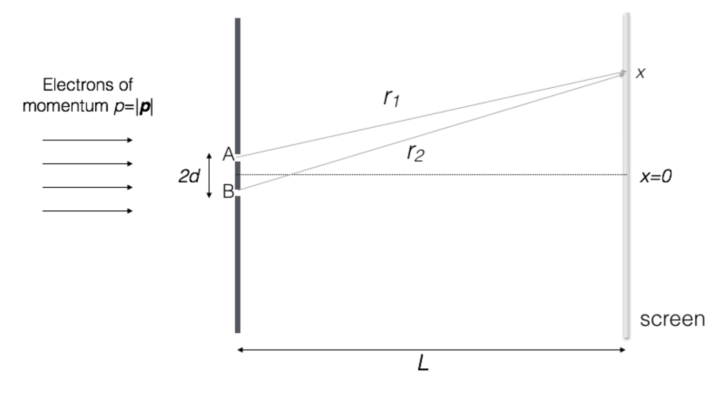
We can assume the wave function that go through the slits and %22%2F%3E%3C%2Fg%3E%3C%2Fg%3E%3Cdefs%3E%3Csymbol%20id%3D%22a%22%20overflow%3D%22visible%22%3E%3Cpath%20d%3D%22M11.34%208.145c0%201.365-1.35%202.1-2.82%202.1H3.54c-.345%200-.495-.015-.495-.36%200-.24.3-.225.48-.225.45-.015.72-.045.795-.06s.105-.06.105-.135c0-.03-.015-.12-.06-.27L2.385%201.23C2.31.9%202.16.705%201.935.63%201.83.6%201.56.585%201.095.585.78.585.63.465.63.225.63.075.78%200%201.095%200H6.39c.975%200%201.875.3%202.73.885.945.645%201.425%201.44%201.425%202.37%200%201.185-.975%201.905-2.04%202.115%201.32.315%202.835%201.32%202.835%202.775M8.31%209.66c1.035%200%201.56-.48%201.56-1.455%200-.765-.3-1.395-.93-1.905a3.25%203.25%200%200%200-2.1-.75H4.755l.9%203.6c.12.51.12.51.75.51Zm.42-5.175c.21-.345.315-.69.315-1.065%200-.78-.3-1.455-.915-2.01S6.825.585%206.03.585H4.005c-.15%200-.255%200-.315.015-.09%200-.135.03-.135.075%200%20.015%200%20.06.015.12A748%20748%200%200%200%204.635%205.1h2.76c.645%200%201.08-.21%201.335-.615%22%2F%3E%3C%2Fsymbol%3E%3C%2Fdefs%3E%3C%2Fsvg%3E) are the same,
and is given by the analogue of plane wave
are the same,
and is given by the analogue of plane wave  .
.
Then, for any point %22%2F%3E%3C%2Fg%3E%3C%2Fg%3E%3Cdefs%3E%3Csymbol%20id%3D%22a%22%20overflow%3D%22visible%22%3E%3Cpath%20d%3D%22M8.325%2010.245h-4.8c-.345%200-.51-.015-.51-.345%200-.165.165-.24.495-.24.3%200%20.9.045.9-.195%200-.03-.015-.12-.06-.27L2.37%201.23C2.28.9%202.13.705%201.92.63%201.815.6%201.545.585%201.08.585.75.585.6.555.6.24.6.075.69%200%20.885%200L2.76.045%203.72.03c.165%200%20.765-.03.96-.03q.36%200%20.36.36c0%20.15-.165.225-.48.225-.6%200-.9.06-.9.195%200%200%20.015.045.045.24l.9%203.66H7.08c.975%200%201.905.3%202.775.885.975.645%201.455%201.44%201.455%202.385%200%201.485-1.41%202.295-2.985%202.295M7.86%209.66c1.305%200%201.95-.45%201.95-1.35%200-.84-.42-1.965-.855-2.355Q8.1%205.19%206.705%205.19h-2.01l.99%203.96c.12.51.12.51.75.51Z%22%2F%3E%3C%2Fsymbol%3E%3C%2Fdefs%3E%3C%2Fsvg%3E) on the screen, the wave function is the superposition of the wave functions from the slits and .
on the screen, the wave function is the superposition of the wave functions from the slits and .
![\begin{align}
\Psi(x, t) &= \psi_A(r_1, t) + \psi_B(r_2, t) \\
&= e^{ikr_1-iwt} + e^{ikr_2-iwt} \\
&= e^{-iwt}\left[\frac{e^{ikr_1}}{r_1} + \frac{e^{ikr_2}}{r_2}\right]
\end{align}](/typst_svg/317ef5a326160d7c2f649fc71fcf9e3091399178.svg)
where %22%2F%3E%3Cuse%20xlink%3Ahref%3D%22%23b%22%20class%3D%22typst-text%22%20transform%3D%22matrix(1%200%200%20-1%207.765%2011.335)%22%2F%3E%3C%2Fg%3E%3C%2Fg%3E%3Cdefs%3E%3Csymbol%20id%3D%22a%22%20overflow%3D%22visible%22%3E%3Cpath%20d%3D%22M6.54%205.61c0%20.63-.615%201.02-1.275%201.02-.735%200-1.35-.345-1.86-1.05-.15.585-.66%201.05-1.365%201.05-.615%200-1.065-.48-1.38-1.455-.15-.495-.225-.78-.225-.87%200-.135.075-.21.24-.21a.27.27%200%200%201%20.165.045c.075.135.12.24.135.345.27%201.14.615%201.71%201.02%201.71.255%200%20.39-.21.39-.63q0-.293-.225-1.215L1.305.945C1.26.75%201.17.36%201.17.285c0-.3.165-.45.48-.45.3%200%20.495.15.6.45l.285%201.08q.248.967.315%201.26l.465%201.92c.03.12.15.315.345.6.405.57.87%201.05%201.605%201.05.18%200%20.33-.03.465-.105-.45-.135-.675-.42-.675-.825%200-.39.21-.585.615-.585.495%200%20.87.435.87.93%22%2F%3E%3C%2Fsymbol%3E%3Csymbol%20id%3D%22b%22%20overflow%3D%22visible%22%3E%3Cpath%20d%3D%22M3.182%206.972c-.452-.441-1.124-.662-2.037-.662v-.46c.619%200%201.112.094%201.49.272V.894c0-.137-.01-.221-.041-.263q-.08-.176-.945-.178h-.431V0l1.869.042L4.967%200v.452h-.431q-.864.002-.955.178c-.022.042-.032.126-.032.262v5.744c0%20.284-.042.336-.367.336%22%2F%3E%3C%2Fsymbol%3E%3C%2Fdefs%3E%3C%2Fsvg%3E) and
and %22%2F%3E%3Cuse%20xlink%3Ahref%3D%22%23b%22%20class%3D%22typst-text%22%20transform%3D%22matrix(1%200%200%20-1%207.765%2011.335)%22%2F%3E%3C%2Fg%3E%3C%2Fg%3E%3Cdefs%3E%3Csymbol%20id%3D%22a%22%20overflow%3D%22visible%22%3E%3Cpath%20d%3D%22M6.54%205.61c0%20.63-.615%201.02-1.275%201.02-.735%200-1.35-.345-1.86-1.05-.15.585-.66%201.05-1.365%201.05-.615%200-1.065-.48-1.38-1.455-.15-.495-.225-.78-.225-.87%200-.135.075-.21.24-.21a.27.27%200%200%201%20.165.045c.075.135.12.24.135.345.27%201.14.615%201.71%201.02%201.71.255%200%20.39-.21.39-.63q0-.293-.225-1.215L1.305.945C1.26.75%201.17.36%201.17.285c0-.3.165-.45.48-.45.3%200%20.495.15.6.45l.285%201.08q.248.967.315%201.26l.465%201.92c.03.12.15.315.345.6.405.57.87%201.05%201.605%201.05.18%200%20.33-.03.465-.105-.45-.135-.675-.42-.675-.825%200-.39.21-.585.615-.585.495%200%20.87.435.87.93%22%2F%3E%3C%2Fsymbol%3E%3Csymbol%20id%3D%22b%22%20overflow%3D%22visible%22%3E%3Cpath%20d%3D%22M1.25%204.452c.335%200%20.587.252.587.588%200%20.378-.199.577-.587.588.23.494.756.892%201.438.892.924%200%201.533-.692%201.533-1.616%200-.505-.178-.988-.546-1.46a5%205%200%200%200-.41-.504L.777.473C.64.347.661.315.661%200h4.326l.326%201.974h-.441c-.074-.556-.157-.882-.252-.955-.053-.032-.378-.053-.997-.053H1.837c.704.62%201.355%201.176%201.974%201.67.473.367.809.692%201.019.976q.473.614.473%201.292c0%20.65-.252%201.165-.767%201.543-.451.346-1.018.525-1.69.525a2.36%202.36%200%200%201-1.502-.504c-.452-.367-.683-.83-.683-1.396%200-.357.263-.62.589-.62%22%2F%3E%3C%2Fsymbol%3E%3C%2Fdefs%3E%3C%2Fsvg%3E) are the distances from the slits and to the point .
And is given by
are the distances from the slits and to the point .
And is given by

Without normalization, the probability density of the wave function is proportional to
![\begin{align}
|\Psi(x, t)|^2 &= \left|\frac{e^{ikr_1}}{r_1} + \frac{e^{ikr_2}}{r_2}\right|^2 \\
&= \frac{1}{r_1^2} + \frac{1}{r_2^2} + \frac{1}{r_1r_2}\left[e^{ik(r_1-r_2)} + e^{-ik(r_1-r_2)}\right] \\
&\approx \frac{1}{L^2}\left[2 + 2\cos(k(r_1-r_2))\right] \\
&= \frac{1}{L^2}\left[2 + 2\cos\left(
k
\left(
\sqrt{L^2 + (x+d)^2} - \sqrt{L^2 + (x-d)^2}
\right)
\right) \right] \\
&= \frac{1}{L^2}\left[2 + 2\cos\left(
k
\frac{
4dx
}{
\sqrt{L^2 + (x+d)^2} + \sqrt{L^2 + (x-d)^2}
}
\right) \right] \\
&\approx \frac{1}{L^2}\left[2 + 2\cos\left(
k
\frac{
4dx
}{
2L
}
\right)\right] \quad\text{As } L \gg x,d \\
&= \frac{1}{L^2}\left[2 + 2\cos\left(
k
\frac{
2dx
}{
L
}
\right)\right]
\end{align}](/typst_svg/8cbcad449aec65b523cf6edc06309db32660528e.svg)
We can see that the probability density of the wave function is proportional to a transformed cosine function, which explains the interference pattern on the screen.
0.7 Parity of TISE Solutions
0.7.1 Even potential and Parity
Given a potential %22%2F%3E%3Cuse%20xlink%3Ahref%3D%22%23b%22%20class%3D%22typst-text%22%20transform%3D%22matrix(1%200%200%20-1%2012.955%2012.22)%22%2F%3E%3Cuse%20xlink%3Ahref%3D%22%23c%22%20class%3D%22typst-text%22%20transform%3D%22matrix(1%200%200%20-1%2018.79%2012.22)%22%2F%3E%3Cuse%20xlink%3Ahref%3D%22%23d%22%20class%3D%22typst-text%22%20transform%3D%22matrix(1%200%200%20-1%2027.37%2012.22)%22%2F%3E%3Cuse%20xlink%3Ahref%3D%22%23e%22%20class%3D%22typst-text%22%20transform%3D%22matrix(1%200%200%20-1%2037.372%2012.22)%22%2F%3E%3Cuse%20xlink%3Ahref%3D%22%23f%22%20class%3D%22typst-text%22%20transform%3D%22matrix(1%200%200%20-1%2045.708%2012.22)%22%2F%3E%3Cuse%20xlink%3Ahref%3D%22%23g%22%20class%3D%22typst-text%22%20transform%3D%22matrix(1%200%200%20-1%2060.705%2012.22)%22%2F%3E%3Cuse%20xlink%3Ahref%3D%22%23h%22%20class%3D%22typst-text%22%20transform%3D%22matrix(1%200%200%20-1%2079.872%2012.22)%22%2F%3E%3C%2Fg%3E%3C%2Fg%3E%3Cdefs%3E%3Csymbol%20id%3D%22a%22%20overflow%3D%22visible%22%3E%3Cpath%20d%3D%22M10.065%2010.2c-.285%200-1.185.045-1.47.045-.225%200-.345-.12-.345-.345%200-.15.105-.225.3-.24.42-.015.63-.165.63-.42%200-.135-.075-.315-.21-.54L4.5%201.605l-.99%207.68c0%20.255.315.375.96.375.3%200%20.435.105.435.36q0%20.225-.27.225c-.33%200-1.5-.045-1.83-.045-.3%200-1.32.045-1.62.045-.225%200-.345-.12-.345-.345%200-.165.15-.24.435-.24.255%200%20.435-.03.555-.06.24-.075.225-.105.27-.39L3.27.06c.045-.255.165-.39.36-.39s.345.105.465.3l5.34%208.49c.345.54.675.885%201.005%201.02.225.105.51.165.84.18.165.015.24.12.255.345.015.165-.075.24-.255.24-.225%200-.99-.045-1.215-.045%22%2F%3E%3C%2Fsymbol%3E%3Csymbol%20id%3D%22b%22%20overflow%3D%22visible%22%3E%3Cpath%20d%3D%22M4.77-3.72c.135%200%20.21.075.21.21%200%20.045-.03.105-.075.165-.78.6-1.41%201.59-1.875%202.955-.405%201.185-.615%202.355-.615%203.51v1.26c0%201.155.21%202.325.615%203.51.465%201.365%201.095%202.355%201.875%202.955a.24.24%200%200%201%20.075.165c0%20.135-.075.21-.21.21a.3.3%200%200%201-.105-.045c-.9-.69-1.65-1.71-2.265-3.075-.585-1.305-.885-2.535-.885-3.72V3.12c0-1.185.3-2.415.885-3.72.615-1.365%201.365-2.385%202.265-3.075a.3.3%200%200%201%20.105-.045%22%2F%3E%3C%2Fsymbol%3E%3Csymbol%20id%3D%22c%22%20overflow%3D%22visible%22%3E%3Cpath%20d%3D%22M7.905%205.595c0%20.69-.675%201.035-1.425%201.035-.645%200-1.155-.345-1.545-1.035-.315.69-.84%201.035-1.605%201.035-.735%200-1.335-.345-1.815-1.02C1.11%205.025.9%204.59.9%204.305c0-.135.075-.21.225-.21.135%200%20.225.075.255.21.285.87.915%201.89%201.92%201.89.495%200%20.735-.315.735-.93%200-.315-.27-1.485-.795-3.495C2.985.765%202.535.27%201.89.27c-.21%200-.405.045-.57.12q.585.225.585.81c0%20.39-.195.585-.6.585-.495%200-.87-.42-.87-.915%200-.69.705-1.035%201.44-1.035.63%200%201.14.345%201.545%201.035.285-.69.825-1.035%201.605-1.035.72%200%201.32.345%201.8%201.02.405.585.615%201.02.615%201.305%200%20.135-.075.21-.225.21-.135%200-.21-.075-.255-.21C6.705%201.305%206.03.27%205.055.27c-.495%200-.75.3-.75.915%200%20.195.075.615.24%201.29l.51%202.025c.285%201.125.75%201.695%201.41%201.695.21%200%20.405-.045.57-.12-.405-.135-.6-.405-.6-.81%200-.39.21-.585.615-.585.48%200%20.855.435.855.915%22%2F%3E%3C%2Fsymbol%3E%3Csymbol%20id%3D%22d%22%20overflow%3D%22visible%22%3E%3Cpath%20d%3D%22M1.17-3.675c.9.69%201.65%201.71%202.265%203.075.585%201.305.885%202.535.885%203.72v1.26c0%201.185-.3%202.415-.885%203.72-.615%201.365-1.365%202.385-2.265%203.075a.3.3%200%200%201-.105.045c-.135%200-.21-.075-.21-.21%200-.06.03-.12.075-.165.78-.6%201.41-1.59%201.875-2.955.405-1.185.615-2.355.615-3.51V3.12c0-1.155-.21-2.325-.615-3.51C2.34-1.755%201.71-2.745.93-3.345c-.045-.06-.075-.12-.075-.165%200-.135.075-.21.21-.21.015%200%20.06.015.105.045%22%2F%3E%3C%2Fsymbol%3E%3Csymbol%20id%3D%22e%22%20overflow%3D%22visible%22%3E%3Cpath%20d%3D%22M2.88%205.625c0%20.45-.345.84-.795.84s-.795-.39-.795-.84.345-.84.795-.84.795.39.795.84m0-4.785c0%20.45-.345.84-.795.84S1.29%201.29%201.29.84%201.635%200%202.085%200s.795.39.795.84%22%2F%3E%3C%2Fsymbol%3E%3Csymbol%20id%3D%22f%22%20overflow%3D%22visible%22%3E%3Cpath%20d%3D%22M1.56%208.85V1.425c0-.75-.075-.78-.855-.78C.39.645.24.54.24.33.24.06.465%200%20.81%200h4.05c.375%200%20.555.105.555.33%200%20.21-.165.315-.48.315-.78%200-.84.03-.84.78V4.65h.435l2.22-3.405c.375-.6.6-.945.66-1.035.09-.135.27-.21.54-.21h2.04c.375%200%20.555.105.555.33%200%20.165-.09.27-.27.3-.375.075-.9.6-1.59%201.56a53%2053%200%200%200-1.8%202.64q2.565.495%202.565%202.61c0%201.005-.45%201.755-1.35%202.22-.78.405-1.665.615-2.64.615H.81c-.375%200-.57-.105-.57-.33%200-.21.15-.315.465-.315.78%200%20.855-.03.855-.78m6.465.105c.525-.315.78-.825.78-1.515%200-1.035-.6-1.665-1.785-1.92.255.42.39%201.05.39%201.905s-.165%201.515-.48%202.01a4%204%200%200%200%201.095-.48M6.78%207.425q0-1.395-.495-1.755c-.33-.24-1.065-.375-2.19-.375v3.6c0%20.555.21.735.855.735%201.425%200%201.83-.705%201.83-2.205M6.195%204.74C7.44%202.76%208.415%201.395%209.15.645H7.875L5.28%204.665a1%201%200%200%200%20.18.015c.21%200%20.45.015.735.06M2.1%209.63h1.5c-.09-.165-.135-.39-.135-.69V1.395c0-.315.03-.57.09-.75H2.1c.06.18.09.435.09.75V8.88c0%20.315-.03.57-.09.75%22%2F%3E%3C%2Fsymbol%3E%3Csymbol%20id%3D%22g%22%20overflow%3D%22visible%22%3E%3Cpath%20d%3D%22M13.98%203.51a.257.257%200%200%201%200%20.48q-1.08.36-2.025%201.53a4.16%204.16%200%200%200-.84%201.845c-.045.195-.165.285-.36.285-.24%200-.36-.12-.36-.375l.015-.03V7.23c.255-1.305.915-2.34%202.01-3.12H1.23q-.36%200-.36-.36t.36-.36h11.19c-1.095-.78-1.755-1.815-2.01-3.12V.255l-.015-.03c0-.255.12-.375.36-.375.195%200%20.315.09.36.285.135.705.42%201.32.84%201.845q.945%201.17%202.025%201.53%22%2F%3E%3C%2Fsymbol%3E%3Csymbol%20id%3D%22h%22%20overflow%3D%22visible%22%3E%3Cpath%20d%3D%22M9.795%201.305c.315.315.48.54.48.66%200%20.24-.12.36-.375.36-.105%200-.21-.075-.345-.225C8.64%201.065%207.485.54%206.09.54c-1.08%200-1.83.48-2.25%201.425-.375.855-.555%201.905-.555%203.15%200%201.125.165%202.13.495%202.985.45%201.215%201.155%201.815%202.1%201.815.675%200%201.335-.27%202.01-.81s1.11-1.14%201.32-1.8c.075-.21.18-.315.345-.315.195%200%20.3.18.3.54v2.475c0%20.375-.105.555-.3.555-.165%200-.285-.12-.345-.345s-.195-.345-.42-.345c-.3%200-.75.12-1.38.345s-1.155.345-1.575.345c-1.365%200-2.55-.42-3.57-1.26-1.14-.93-1.71-2.31-1.71-4.155S1.125%201.905%202.25.99C3.285.135%204.5-.285%205.865-.285c1.515%200%202.835.525%203.93%201.59M9.225%209.3v-.645q-.18.202-.54.585h.12c.165%200%20.315.015.42.06m-5.385.225A3.6%203.6%200%200%201%203.465%209C3%208.235%202.64%206.435%202.64%205.115c0-2.07.45-3.54%201.35-4.425-1.875.72-2.805%202.205-2.805%204.44%200%202.22.885%203.69%202.655%204.395%22%2F%3E%3C%2Fsymbol%3E%3C%2Fdefs%3E%3C%2Fsvg%3E) , the potential is said to be even if
, the potential is said to be even if
%22%2F%3E%3Cuse%20xlink%3Ahref%3D%22%23b%22%20class%3D%22typst-text%22%20transform%3D%22matrix(1%200%200%20-1%2021.955%2021.22)%22%2F%3E%3Cuse%20xlink%3Ahref%3D%22%23c%22%20class%3D%22typst-text%22%20transform%3D%22matrix(1%200%200%20-1%2027.79%2021.22)%22%2F%3E%3Cuse%20xlink%3Ahref%3D%22%23d%22%20class%3D%22typst-text%22%20transform%3D%22matrix(1%200%200%20-1%2036.37%2021.22)%22%2F%3E%3Cuse%20xlink%3Ahref%3D%22%23e%22%20class%3D%22typst-text%22%20transform%3D%22matrix(1%200%200%20-1%2046.372%2021.22)%22%2F%3E%3Cuse%20xlink%3Ahref%3D%22%23a%22%20class%3D%22typst-text%22%20transform%3D%22matrix(1%200%200%20-1%2062.208%2021.22)%22%2F%3E%3Cuse%20xlink%3Ahref%3D%22%23b%22%20class%3D%22typst-text%22%20transform%3D%22matrix(1%200%200%20-1%2074.163%2021.22)%22%2F%3E%3Cuse%20xlink%3Ahref%3D%22%23f%22%20class%3D%22typst-text%22%20transform%3D%22matrix(1%200%200%20-1%2079.998%2021.22)%22%2F%3E%3Cuse%20xlink%3Ahref%3D%22%23c%22%20class%3D%22typst-text%22%20transform%3D%22matrix(1%200%200%20-1%2091.668%2021.22)%22%2F%3E%3Cuse%20xlink%3Ahref%3D%22%23d%22%20class%3D%22typst-text%22%20transform%3D%22matrix(1%200%200%20-1%20100.248%2021.22)%22%2F%3E%3C%2Fg%3E%3C%2Fg%3E%3Cdefs%3E%3Csymbol%20id%3D%22a%22%20overflow%3D%22visible%22%3E%3Cpath%20d%3D%22M10.065%2010.2c-.285%200-1.185.045-1.47.045-.225%200-.345-.12-.345-.345%200-.15.105-.225.3-.24.42-.015.63-.165.63-.42%200-.135-.075-.315-.21-.54L4.5%201.605l-.99%207.68c0%20.255.315.375.96.375.3%200%20.435.105.435.36q0%20.225-.27.225c-.33%200-1.5-.045-1.83-.045-.3%200-1.32.045-1.62.045-.225%200-.345-.12-.345-.345%200-.165.15-.24.435-.24.255%200%20.435-.03.555-.06.24-.075.225-.105.27-.39L3.27.06c.045-.255.165-.39.36-.39s.345.105.465.3l5.34%208.49c.345.54.675.885%201.005%201.02.225.105.51.165.84.18.165.015.24.12.255.345.015.165-.075.24-.255.24-.225%200-.99-.045-1.215-.045%22%2F%3E%3C%2Fsymbol%3E%3Csymbol%20id%3D%22b%22%20overflow%3D%22visible%22%3E%3Cpath%20d%3D%22M4.77-3.72c.135%200%20.21.075.21.21%200%20.045-.03.105-.075.165-.78.6-1.41%201.59-1.875%202.955-.405%201.185-.615%202.355-.615%203.51v1.26c0%201.155.21%202.325.615%203.51.465%201.365%201.095%202.355%201.875%202.955a.24.24%200%200%201%20.075.165c0%20.135-.075.21-.21.21a.3.3%200%200%201-.105-.045c-.9-.69-1.65-1.71-2.265-3.075-.585-1.305-.885-2.535-.885-3.72V3.12c0-1.185.3-2.415.885-3.72.615-1.365%201.365-2.385%202.265-3.075a.3.3%200%200%201%20.105-.045%22%2F%3E%3C%2Fsymbol%3E%3Csymbol%20id%3D%22c%22%20overflow%3D%22visible%22%3E%3Cpath%20d%3D%22M7.905%205.595c0%20.69-.675%201.035-1.425%201.035-.645%200-1.155-.345-1.545-1.035-.315.69-.84%201.035-1.605%201.035-.735%200-1.335-.345-1.815-1.02C1.11%205.025.9%204.59.9%204.305c0-.135.075-.21.225-.21.135%200%20.225.075.255.21.285.87.915%201.89%201.92%201.89.495%200%20.735-.315.735-.93%200-.315-.27-1.485-.795-3.495C2.985.765%202.535.27%201.89.27c-.21%200-.405.045-.57.12q.585.225.585.81c0%20.39-.195.585-.6.585-.495%200-.87-.42-.87-.915%200-.69.705-1.035%201.44-1.035.63%200%201.14.345%201.545%201.035.285-.69.825-1.035%201.605-1.035.72%200%201.32.345%201.8%201.02.405.585.615%201.02.615%201.305%200%20.135-.075.21-.225.21-.135%200-.21-.075-.255-.21C6.705%201.305%206.03.27%205.055.27c-.495%200-.75.3-.75.915%200%20.195.075.615.24%201.29l.51%202.025c.285%201.125.75%201.695%201.41%201.695.21%200%20.405-.045.57-.12-.405-.135-.6-.405-.6-.81%200-.39.21-.585.615-.585.48%200%20.855.435.855.915%22%2F%3E%3C%2Fsymbol%3E%3Csymbol%20id%3D%22d%22%20overflow%3D%22visible%22%3E%3Cpath%20d%3D%22M1.17-3.675c.9.69%201.65%201.71%202.265%203.075.585%201.305.885%202.535.885%203.72v1.26c0%201.185-.3%202.415-.885%203.72-.615%201.365-1.365%202.385-2.265%203.075a.3.3%200%200%201-.105.045c-.135%200-.21-.075-.21-.21%200-.06.03-.12.075-.165.78-.6%201.41-1.59%201.875-2.955.405-1.185.615-2.355.615-3.51V3.12c0-1.155-.21-2.325-.615-3.51C2.34-1.755%201.71-2.745.93-3.345c-.045-.06-.075-.12-.075-.165%200-.135.075-.21.21-.21.015%200%20.06.015.105.045%22%2F%3E%3C%2Fsymbol%3E%3Csymbol%20id%3D%22e%22%20overflow%3D%22visible%22%3E%3Cpath%20d%3D%22M10.47%205.505H1.2c-.24%200-.36-.12-.36-.345s.12-.345.36-.345h9.27c.24%200%20.36.12.36.345%200%20.18-.165.345-.36.345m0-2.82H1.2c-.24%200-.36-.12-.36-.345s.12-.345.36-.345h9.27c.24%200%20.36.12.36.345a.35.35%200%200%201-.36.345%22%2F%3E%3C%2Fsymbol%3E%3Csymbol%20id%3D%22f%22%20overflow%3D%22visible%22%3E%3Cpath%20d%3D%22M10.47%204.05H1.2c-.24%200-.36-.105-.36-.3s.12-.3.36-.3h9.27c.24%200%20.36.105.36.3%200%20.18-.18.3-.36.3%22%2F%3E%3C%2Fsymbol%3E%3C%2Fdefs%3E%3C%2Fsvg%3E)
In such cases, we can assume the TISE solution has definite parity, that is:
%22%2F%3E%3Cuse%20xlink%3Ahref%3D%22%23b%22%20class%3D%22typst-text%22%20transform%3D%22matrix(1%200%200%20-1%2019.015%2021.22)%22%2F%3E%3Cuse%20xlink%3Ahref%3D%22%23c%22%20class%3D%22typst-text%22%20transform%3D%22matrix(1%200%200%20-1%2024.85%2021.22)%22%2F%3E%3Cuse%20xlink%3Ahref%3D%22%23d%22%20class%3D%22typst-text%22%20transform%3D%22matrix(1%200%200%20-1%2033.43%2021.22)%22%2F%3E%3Cuse%20xlink%3Ahref%3D%22%23e%22%20class%3D%22typst-text%22%20transform%3D%22matrix(1%200%200%20-1%2043.432%2021.22)%22%2F%3E%3Cuse%20xlink%3Ahref%3D%22%23f%22%20class%3D%22typst-text%22%20transform%3D%22matrix(1%200%200%20-1%2059.268%2021.22)%22%2F%3E%3Cuse%20xlink%3Ahref%3D%22%23a%22%20class%3D%22typst-text%22%20transform%3D%22matrix(1%200%200%20-1%2070.938%2021.22)%22%2F%3E%3Cuse%20xlink%3Ahref%3D%22%23b%22%20class%3D%22typst-text%22%20transform%3D%22matrix(1%200%200%20-1%2079.953%2021.22)%22%2F%3E%3Cuse%20xlink%3Ahref%3D%22%23g%22%20class%3D%22typst-text%22%20transform%3D%22matrix(1%200%200%20-1%2085.788%2021.22)%22%2F%3E%3Cuse%20xlink%3Ahref%3D%22%23c%22%20class%3D%22typst-text%22%20transform%3D%22matrix(1%200%200%20-1%2097.458%2021.22)%22%2F%3E%3Cuse%20xlink%3Ahref%3D%22%23d%22%20class%3D%22typst-text%22%20transform%3D%22matrix(1%200%200%20-1%20106.038%2021.22)%22%2F%3E%3C%2Fg%3E%3C%2Fg%3E%3Cdefs%3E%3Csymbol%20id%3D%22a%22%20overflow%3D%22visible%22%3E%3Cpath%20d%3D%22M5.775%206.675c.285%201.185.585%202.34.855%203.525v.045c-.045.105-.12.165-.24.165-.135%200-.225-.12-.27-.345l-.855-3.39C4.14%206.63%203.12%206.21%202.205%205.43%201.23%204.605.735%203.645.735%202.55.735.93%201.98-.105%203.555-.195c-.285-1.185-.495-2.04-.63-2.55-.015-.045-.015-.09-.015-.105%200-.15.075-.225.24-.225s.21.09.255.27l.66%202.595c1.125.045%202.145.465%203.06%201.245.975.84%201.47%201.8%201.47%202.895%200%201.605-1.275%202.61-2.82%202.745m-.12-.45c1.14-.075%201.86-.78%201.86-1.98%200-.6-.135-1.2-.405-1.785C6.63%201.38%205.535.39%204.17.255Zm-3.84-3.99c0%20.6.135%201.2.405%201.785.48%201.08%201.575%202.055%202.925%202.205L3.66.24c-1.125.09-1.845.795-1.845%201.995%22%2F%3E%3C%2Fsymbol%3E%3Csymbol%20id%3D%22b%22%20overflow%3D%22visible%22%3E%3Cpath%20d%3D%22M4.77-3.72c.135%200%20.21.075.21.21%200%20.045-.03.105-.075.165-.78.6-1.41%201.59-1.875%202.955-.405%201.185-.615%202.355-.615%203.51v1.26c0%201.155.21%202.325.615%203.51.465%201.365%201.095%202.355%201.875%202.955a.24.24%200%200%201%20.075.165c0%20.135-.075.21-.21.21a.3.3%200%200%201-.105-.045c-.9-.69-1.65-1.71-2.265-3.075-.585-1.305-.885-2.535-.885-3.72V3.12c0-1.185.3-2.415.885-3.72.615-1.365%201.365-2.385%202.265-3.075a.3.3%200%200%201%20.105-.045%22%2F%3E%3C%2Fsymbol%3E%3Csymbol%20id%3D%22c%22%20overflow%3D%22visible%22%3E%3Cpath%20d%3D%22M7.905%205.595c0%20.69-.675%201.035-1.425%201.035-.645%200-1.155-.345-1.545-1.035-.315.69-.84%201.035-1.605%201.035-.735%200-1.335-.345-1.815-1.02C1.11%205.025.9%204.59.9%204.305c0-.135.075-.21.225-.21.135%200%20.225.075.255.21.285.87.915%201.89%201.92%201.89.495%200%20.735-.315.735-.93%200-.315-.27-1.485-.795-3.495C2.985.765%202.535.27%201.89.27c-.21%200-.405.045-.57.12q.585.225.585.81c0%20.39-.195.585-.6.585-.495%200-.87-.42-.87-.915%200-.69.705-1.035%201.44-1.035.63%200%201.14.345%201.545%201.035.285-.69.825-1.035%201.605-1.035.72%200%201.32.345%201.8%201.02.405.585.615%201.02.615%201.305%200%20.135-.075.21-.225.21-.135%200-.21-.075-.255-.21C6.705%201.305%206.03.27%205.055.27c-.495%200-.75.3-.75.915%200%20.195.075.615.24%201.29l.51%202.025c.285%201.125.75%201.695%201.41%201.695.21%200%20.405-.045.57-.12-.405-.135-.6-.405-.6-.81%200-.39.21-.585.615-.585.48%200%20.855.435.855.915%22%2F%3E%3C%2Fsymbol%3E%3Csymbol%20id%3D%22d%22%20overflow%3D%22visible%22%3E%3Cpath%20d%3D%22M1.17-3.675c.9.69%201.65%201.71%202.265%203.075.585%201.305.885%202.535.885%203.72v1.26c0%201.185-.3%202.415-.885%203.72-.615%201.365-1.365%202.385-2.265%203.075a.3.3%200%200%201-.105.045c-.135%200-.21-.075-.21-.21%200-.06.03-.12.075-.165.78-.6%201.41-1.59%201.875-2.955.405-1.185.615-2.355.615-3.51V3.12c0-1.155-.21-2.325-.615-3.51C2.34-1.755%201.71-2.745.93-3.345c-.045-.06-.075-.12-.075-.165%200-.135.075-.21.21-.21.015%200%20.06.015.105.045%22%2F%3E%3C%2Fsymbol%3E%3Csymbol%20id%3D%22e%22%20overflow%3D%22visible%22%3E%3Cpath%20d%3D%22M10.47%205.505H1.2c-.24%200-.36-.12-.36-.345s.12-.345.36-.345h9.27c.24%200%20.36.12.36.345%200%20.18-.165.345-.36.345m0-2.82H1.2c-.24%200-.36-.12-.36-.345s.12-.345.36-.345h9.27c.24%200%20.36.12.36.345a.35.35%200%200%201-.36.345%22%2F%3E%3C%2Fsymbol%3E%3Csymbol%20id%3D%22f%22%20overflow%3D%22visible%22%3E%3Cpath%20d%3D%22M10.47-.555H6.195V3.39h4.275q.36%200%20.36.36t-.36.36H6.195v4.275q0%20.36-.36.36t-.36-.36V4.11H1.2q-.36%200-.36-.36t.36-.36h4.275V-.555H1.2C.96-.555.84-.675.84-.9q0-.36.36-.36h9.27q.36%200%20.36.36c0%20.18-.165.345-.36.345%22%2F%3E%3C%2Fsymbol%3E%3Csymbol%20id%3D%22g%22%20overflow%3D%22visible%22%3E%3Cpath%20d%3D%22M10.47%204.05H1.2c-.24%200-.36-.105-.36-.3s.12-.3.36-.3h9.27c.24%200%20.36.105.36.3%200%20.18-.18.3-.36.3%22%2F%3E%3C%2Fsymbol%3E%3C%2Fdefs%3E%3C%2Fsvg%3E)
0.7.2 Real Potential and Parity
Given a real potential %22%2F%3E%3Cuse%20xlink%3Ahref%3D%22%23b%22%20class%3D%22typst-text%22%20transform%3D%22matrix(1%200%200%20-1%2012.955%2012.22)%22%2F%3E%3Cuse%20xlink%3Ahref%3D%22%23c%22%20class%3D%22typst-text%22%20transform%3D%22matrix(1%200%200%20-1%2018.79%2012.22)%22%2F%3E%3Cuse%20xlink%3Ahref%3D%22%23d%22%20class%3D%22typst-text%22%20transform%3D%22matrix(1%200%200%20-1%2027.37%2012.22)%22%2F%3E%3C%2Fg%3E%3C%2Fg%3E%3Cdefs%3E%3Csymbol%20id%3D%22a%22%20overflow%3D%22visible%22%3E%3Cpath%20d%3D%22M10.065%2010.2c-.285%200-1.185.045-1.47.045-.225%200-.345-.12-.345-.345%200-.15.105-.225.3-.24.42-.015.63-.165.63-.42%200-.135-.075-.315-.21-.54L4.5%201.605l-.99%207.68c0%20.255.315.375.96.375.3%200%20.435.105.435.36q0%20.225-.27.225c-.33%200-1.5-.045-1.83-.045-.3%200-1.32.045-1.62.045-.225%200-.345-.12-.345-.345%200-.165.15-.24.435-.24.255%200%20.435-.03.555-.06.24-.075.225-.105.27-.39L3.27.06c.045-.255.165-.39.36-.39s.345.105.465.3l5.34%208.49c.345.54.675.885%201.005%201.02.225.105.51.165.84.18.165.015.24.12.255.345.015.165-.075.24-.255.24-.225%200-.99-.045-1.215-.045%22%2F%3E%3C%2Fsymbol%3E%3Csymbol%20id%3D%22b%22%20overflow%3D%22visible%22%3E%3Cpath%20d%3D%22M4.77-3.72c.135%200%20.21.075.21.21%200%20.045-.03.105-.075.165-.78.6-1.41%201.59-1.875%202.955-.405%201.185-.615%202.355-.615%203.51v1.26c0%201.155.21%202.325.615%203.51.465%201.365%201.095%202.355%201.875%202.955a.24.24%200%200%201%20.075.165c0%20.135-.075.21-.21.21a.3.3%200%200%201-.105-.045c-.9-.69-1.65-1.71-2.265-3.075-.585-1.305-.885-2.535-.885-3.72V3.12c0-1.185.3-2.415.885-3.72.615-1.365%201.365-2.385%202.265-3.075a.3.3%200%200%201%20.105-.045%22%2F%3E%3C%2Fsymbol%3E%3Csymbol%20id%3D%22c%22%20overflow%3D%22visible%22%3E%3Cpath%20d%3D%22M7.905%205.595c0%20.69-.675%201.035-1.425%201.035-.645%200-1.155-.345-1.545-1.035-.315.69-.84%201.035-1.605%201.035-.735%200-1.335-.345-1.815-1.02C1.11%205.025.9%204.59.9%204.305c0-.135.075-.21.225-.21.135%200%20.225.075.255.21.285.87.915%201.89%201.92%201.89.495%200%20.735-.315.735-.93%200-.315-.27-1.485-.795-3.495C2.985.765%202.535.27%201.89.27c-.21%200-.405.045-.57.12q.585.225.585.81c0%20.39-.195.585-.6.585-.495%200-.87-.42-.87-.915%200-.69.705-1.035%201.44-1.035.63%200%201.14.345%201.545%201.035.285-.69.825-1.035%201.605-1.035.72%200%201.32.345%201.8%201.02.405.585.615%201.02.615%201.305%200%20.135-.075.21-.225.21-.135%200-.21-.075-.255-.21C6.705%201.305%206.03.27%205.055.27c-.495%200-.75.3-.75.915%200%20.195.075.615.24%201.29l.51%202.025c.285%201.125.75%201.695%201.41%201.695.21%200%20.405-.045.57-.12-.405-.135-.6-.405-.6-.81%200-.39.21-.585.615-.585.48%200%20.855.435.855.915%22%2F%3E%3C%2Fsymbol%3E%3Csymbol%20id%3D%22d%22%20overflow%3D%22visible%22%3E%3Cpath%20d%3D%22M1.17-3.675c.9.69%201.65%201.71%202.265%203.075.585%201.305.885%202.535.885%203.72v1.26c0%201.185-.3%202.415-.885%203.72-.615%201.365-1.365%202.385-2.265%203.075a.3.3%200%200%201-.105.045c-.135%200-.21-.075-.21-.21%200-.06.03-.12.075-.165.78-.6%201.41-1.59%201.875-2.955.405-1.185.615-2.355.615-3.51V3.12c0-1.155-.21-2.325-.615-3.51C2.34-1.755%201.71-2.745.93-3.345c-.045-.06-.075-.12-.075-.165%200-.135.075-.21.21-.21.015%200%20.06.015.105.045%22%2F%3E%3C%2Fsymbol%3E%3C%2Fdefs%3E%3C%2Fsvg%3E) , we can assume the TISE solution to have definite parity regarding conjugation, that is:
, we can assume the TISE solution to have definite parity regarding conjugation, that is:
%22%2F%3E%3Cuse%20xlink%3Ahref%3D%22%23b%22%20class%3D%22typst-text%22%20transform%3D%22matrix(1%200%200%20-1%2019.015%2023.32)%22%2F%3E%3Cuse%20xlink%3Ahref%3D%22%23c%22%20class%3D%22typst-text%22%20transform%3D%22matrix(1%200%200%20-1%2024.85%2023.32)%22%2F%3E%3Cuse%20xlink%3Ahref%3D%22%23d%22%20class%3D%22typst-text%22%20transform%3D%22matrix(1%200%200%20-1%2033.43%2023.32)%22%2F%3E%3Cuse%20xlink%3Ahref%3D%22%23e%22%20class%3D%22typst-text%22%20transform%3D%22matrix(1%200%200%20-1%2043.432%2023.32)%22%2F%3E%3Cuse%20xlink%3Ahref%3D%22%23a%22%20class%3D%22typst-text%22%20transform%3D%22matrix(1%200%200%20-1%2059.268%2023.32)%22%2F%3E%3Cuse%20xlink%3Ahref%3D%22%23f%22%20class%3D%22typst-text%22%20transform%3D%22matrix(1%200%200%20-1%2068.283%2017.875)%22%2F%3E%3Cuse%20xlink%3Ahref%3D%22%23b%22%20class%3D%22typst-text%22%20transform%3D%22matrix(1%200%200%20-1%2074.373%2023.32)%22%2F%3E%3Cuse%20xlink%3Ahref%3D%22%23c%22%20class%3D%22typst-text%22%20transform%3D%22matrix(1%200%200%20-1%2080.208%2023.32)%22%2F%3E%3Cuse%20xlink%3Ahref%3D%22%23d%22%20class%3D%22typst-text%22%20transform%3D%22matrix(1%200%200%20-1%2088.788%2023.32)%22%2F%3E%3C%2Fg%3E%3C%2Fg%3E%3Cdefs%3E%3Csymbol%20id%3D%22a%22%20overflow%3D%22visible%22%3E%3Cpath%20d%3D%22M5.775%206.675c.285%201.185.585%202.34.855%203.525v.045c-.045.105-.12.165-.24.165-.135%200-.225-.12-.27-.345l-.855-3.39C4.14%206.63%203.12%206.21%202.205%205.43%201.23%204.605.735%203.645.735%202.55.735.93%201.98-.105%203.555-.195c-.285-1.185-.495-2.04-.63-2.55-.015-.045-.015-.09-.015-.105%200-.15.075-.225.24-.225s.21.09.255.27l.66%202.595c1.125.045%202.145.465%203.06%201.245.975.84%201.47%201.8%201.47%202.895%200%201.605-1.275%202.61-2.82%202.745m-.12-.45c1.14-.075%201.86-.78%201.86-1.98%200-.6-.135-1.2-.405-1.785C6.63%201.38%205.535.39%204.17.255Zm-3.84-3.99c0%20.6.135%201.2.405%201.785.48%201.08%201.575%202.055%202.925%202.205L3.66.24c-1.125.09-1.845.795-1.845%201.995%22%2F%3E%3C%2Fsymbol%3E%3Csymbol%20id%3D%22b%22%20overflow%3D%22visible%22%3E%3Cpath%20d%3D%22M4.77-3.72c.135%200%20.21.075.21.21%200%20.045-.03.105-.075.165-.78.6-1.41%201.59-1.875%202.955-.405%201.185-.615%202.355-.615%203.51v1.26c0%201.155.21%202.325.615%203.51.465%201.365%201.095%202.355%201.875%202.955a.24.24%200%200%201%20.075.165c0%20.135-.075.21-.21.21a.3.3%200%200%201-.105-.045c-.9-.69-1.65-1.71-2.265-3.075-.585-1.305-.885-2.535-.885-3.72V3.12c0-1.185.3-2.415.885-3.72.615-1.365%201.365-2.385%202.265-3.075a.3.3%200%200%201%20.105-.045%22%2F%3E%3C%2Fsymbol%3E%3Csymbol%20id%3D%22c%22%20overflow%3D%22visible%22%3E%3Cpath%20d%3D%22M7.905%205.595c0%20.69-.675%201.035-1.425%201.035-.645%200-1.155-.345-1.545-1.035-.315.69-.84%201.035-1.605%201.035-.735%200-1.335-.345-1.815-1.02C1.11%205.025.9%204.59.9%204.305c0-.135.075-.21.225-.21.135%200%20.225.075.255.21.285.87.915%201.89%201.92%201.89.495%200%20.735-.315.735-.93%200-.315-.27-1.485-.795-3.495C2.985.765%202.535.27%201.89.27c-.21%200-.405.045-.57.12q.585.225.585.81c0%20.39-.195.585-.6.585-.495%200-.87-.42-.87-.915%200-.69.705-1.035%201.44-1.035.63%200%201.14.345%201.545%201.035.285-.69.825-1.035%201.605-1.035.72%200%201.32.345%201.8%201.02.405.585.615%201.02.615%201.305%200%20.135-.075.21-.225.21-.135%200-.21-.075-.255-.21C6.705%201.305%206.03.27%205.055.27c-.495%200-.75.3-.75.915%200%20.195.075.615.24%201.29l.51%202.025c.285%201.125.75%201.695%201.41%201.695.21%200%20.405-.045.57-.12-.405-.135-.6-.405-.6-.81%200-.39.21-.585.615-.585.48%200%20.855.435.855.915%22%2F%3E%3C%2Fsymbol%3E%3Csymbol%20id%3D%22d%22%20overflow%3D%22visible%22%3E%3Cpath%20d%3D%22M1.17-3.675c.9.69%201.65%201.71%202.265%203.075.585%201.305.885%202.535.885%203.72v1.26c0%201.185-.3%202.415-.885%203.72-.615%201.365-1.365%202.385-2.265%203.075a.3.3%200%200%201-.105.045c-.135%200-.21-.075-.21-.21%200-.06.03-.12.075-.165.78-.6%201.41-1.59%201.875-2.955.405-1.185.615-2.355.615-3.51V3.12c0-1.155-.21-2.325-.615-3.51C2.34-1.755%201.71-2.745.93-3.345c-.045-.06-.075-.12-.075-.165%200-.135.075-.21.21-.21.015%200%20.06.015.105.045%22%2F%3E%3C%2Fsymbol%3E%3Csymbol%20id%3D%22e%22%20overflow%3D%22visible%22%3E%3Cpath%20d%3D%22M10.47%205.505H1.2c-.24%200-.36-.12-.36-.345s.12-.345.36-.345h9.27c.24%200%20.36.12.36.345%200%20.18-.165.345-.36.345m0-2.82H1.2c-.24%200-.36-.12-.36-.345s.12-.345.36-.345h9.27c.24%200%20.36.12.36.345a.35.35%200%200%201-.36.345%22%2F%3E%3C%2Fsymbol%3E%3Csymbol%20id%3D%22f%22%20overflow%3D%22visible%22%3E%3Cpath%20d%3D%22M4.62%204.673a.315.315%200%200%201-.2.304l-1.449.64%201.45.641a.32.32%200%200%201%20.199.315.35.35%200%200%201-.346.346.32.32%200%200%201-.2-.063l-1.27-.934.157%201.565a.33.33%200%200%201-.336.388.33.33%200%200%201-.336-.388l.157-1.565-1.27.934a.3.3%200%200%201-.262.064C.724%206.867.63%206.752.63%206.563c0-.137.063-.242.2-.305l1.449-.64-1.45-.641a.32.32%200%200%201-.199-.315c0-.189.168-.346.357-.346q.11%200%20.189.063l1.27.934-.157-1.565a.33.33%200%200%201%20.336-.388.33.33%200%200%201%20.336.388l-.157%201.565%201.27-.934a.32.32%200%200%201%20.2-.063c.189%200%20.346.168.346.357%22%2F%3E%3C%2Fsymbol%3E%3C%2Fdefs%3E%3C%2Fsvg%3E)
0.8 States of TISE Solutions
In general there are three kinds of states of TISE solutions:
- Bound States
- Scattering States
- Non-physical States
0.8.1 Bound States
Bound states are states where the energy eigenvalue is less than the potential energy at infinity and greater than the minimum potential energy.
In such cases, the TISE solution is normalizable, and the energy eigenvalue is quantized.
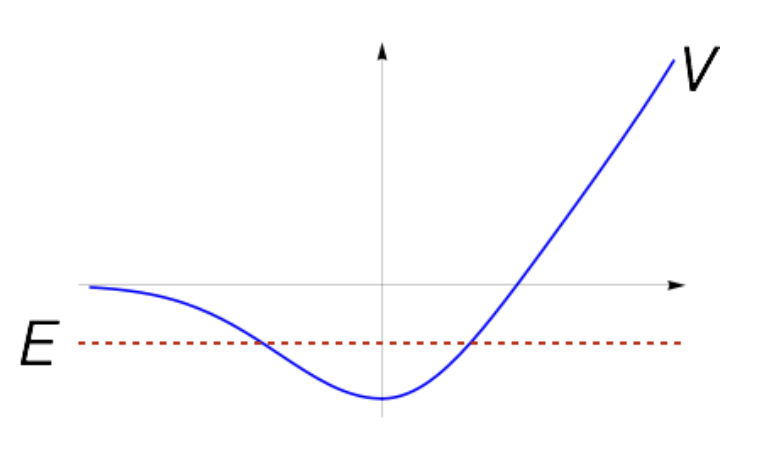
0.8.2 Scattering States
Scattering states are states where the energy eigenvalue is greater than the potential energy at infinity.
In such cases, the TISE solution is not normalizable, and the energy eigenvalue is continuous.
Scattering states can be approximated by normalizable states by similar method as the classical plane wave.
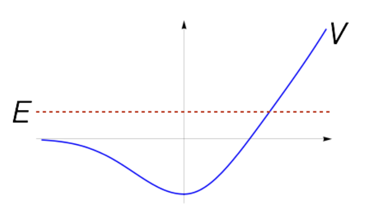
0.8.3 Non-physical States
Non-physical states are states where the energy eigenvalue is less than the minimum potential energy.
This case cannot happen in real physical systems.
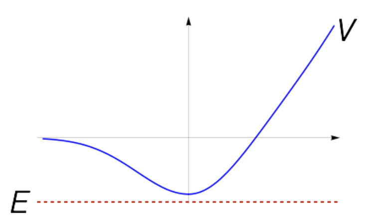
0.9 Continuity Equation and Probability Current
Consider the potential to be real. Define the probability density of a wave function %22%2F%3E%3Cuse%20xlink%3Ahref%3D%22%23b%22%20class%3D%22typst-text%22%20transform%3D%22matrix(1%200%200%20-1%2016.897%2012.22)%22%2F%3E%3Cuse%20xlink%3Ahref%3D%22%23c%22%20class%3D%22typst-text%22%20transform%3D%22matrix(1%200%200%20-1%2032.733%2012.22)%22%2F%3E%3Cuse%20xlink%3Ahref%3D%22%23d%22%20class%3D%22typst-text%22%20transform%3D%22matrix(1%200%200%20-1%2044.403%2012.22)%22%2F%3E%3Cuse%20xlink%3Ahref%3D%22%23e%22%20class%3D%22typst-text%22%20transform%3D%22matrix(1%200%200%20-1%2050.238%2012.22)%22%2F%3E%3Cuse%20xlink%3Ahref%3D%22%23f%22%20class%3D%22typst-text%22%20transform%3D%22matrix(1%200%200%20-1%2058.818%2012.22)%22%2F%3E%3Cuse%20xlink%3Ahref%3D%22%23g%22%20class%3D%22typst-text%22%20transform%3D%22matrix(1%200%200%20-1%2065.488%2012.22)%22%2F%3E%3Cuse%20xlink%3Ahref%3D%22%23h%22%20class%3D%22typst-text%22%20transform%3D%22matrix(1%200%200%20-1%2070.903%2012.22)%22%2F%3E%3C%2Fg%3E%3C%2Fg%3E%3Cdefs%3E%3Csymbol%20id%3D%22a%22%20overflow%3D%22visible%22%3E%3Cpath%20d%3D%22M8.325%2010.245h-4.8c-.345%200-.51-.015-.51-.345%200-.165.165-.24.495-.24.3%200%20.9.045.9-.195%200-.03-.015-.12-.06-.27L2.37%201.23C2.28.9%202.13.705%201.92.63%201.815.6%201.545.585%201.08.585.75.585.6.555.6.24.6.075.69%200%20.885%200L2.76.045%203.72.03c.165%200%20.765-.03.96-.03q.36%200%20.36.36c0%20.15-.165.225-.48.225-.6%200-.9.06-.9.195%200%200%20.015.045.045.24l.9%203.66H7.08c.975%200%201.905.3%202.775.885.975.645%201.455%201.44%201.455%202.385%200%201.485-1.41%202.295-2.985%202.295M7.86%209.66c1.305%200%201.95-.45%201.95-1.35%200-.84-.42-1.965-.855-2.355Q8.1%205.19%206.705%205.19h-2.01l.99%203.96c.12.51.12.51.75.51Z%22%2F%3E%3C%2Fsymbol%3E%3Csymbol%20id%3D%22b%22%20overflow%3D%22visible%22%3E%3Cpath%20d%3D%22M10.47%205.505H1.2c-.24%200-.36-.12-.36-.345s.12-.345.36-.345h9.27c.24%200%20.36.12.36.345%200%20.18-.165.345-.36.345m0-2.82H1.2c-.24%200-.36-.12-.36-.345s.12-.345.36-.345h9.27c.24%200%20.36.12.36.345a.35.35%200%200%201-.36.345%22%2F%3E%3C%2Fsymbol%3E%3Csymbol%20id%3D%22c%22%20overflow%3D%22visible%22%3E%3Cpath%20d%3D%22M5.115%202.01v-.78c0-.195-.015-.315-.06-.39C4.98.675%204.56.585%203.765.585H3.21V0q.607.045%202.565.045C7.095.045%207.95.03%208.355%200v.585H7.8c-.795%200-1.215.075-1.29.24-.045.075-.06.21-.06.405v.78c2.235.285%203.345%201.71%203.345%204.275%200%20.195.03.48.105.855.075.45.3.705.66.75.165.015.24.09.24.225s-.135.21-.42.21h-.555c-.3%200-.54-.06-.735-.165-.42-.27-.63-.99-.645-2.145-.015-1.98-.69-3.15-1.995-3.51v6.51c0%20.195.015.315.06.39.075.165.495.255%201.29.255h.555v.585Q7.748%2010.2%205.79%2010.2c-1.32%200-2.175.015-2.58.045V9.66h.555c.795%200%201.215-.075%201.29-.24.045-.075.06-.21.06-.405v-6.51C3.84%202.88%203.21%204.11%203.21%206.195c0%201.425-.465%202.13-1.38%202.13h-.54c-.285%200-.435-.075-.435-.21q0-.18.18-.225a.8.8%200%200%200%20.42-.15c.27-.21.405-.81.405-1.815%200-2.205%201.275-3.63%203.255-3.915%22%2F%3E%3C%2Fsymbol%3E%3Csymbol%20id%3D%22d%22%20overflow%3D%22visible%22%3E%3Cpath%20d%3D%22M4.77-3.72c.135%200%20.21.075.21.21%200%20.045-.03.105-.075.165-.78.6-1.41%201.59-1.875%202.955-.405%201.185-.615%202.355-.615%203.51v1.26c0%201.155.21%202.325.615%203.51.465%201.365%201.095%202.355%201.875%202.955a.24.24%200%200%201%20.075.165c0%20.135-.075.21-.21.21a.3.3%200%200%201-.105-.045c-.9-.69-1.65-1.71-2.265-3.075-.585-1.305-.885-2.535-.885-3.72V3.12c0-1.185.3-2.415.885-3.72.615-1.365%201.365-2.385%202.265-3.075a.3.3%200%200%201%20.105-.045%22%2F%3E%3C%2Fsymbol%3E%3Csymbol%20id%3D%22e%22%20overflow%3D%22visible%22%3E%3Cpath%20d%3D%22M7.905%205.595c0%20.69-.675%201.035-1.425%201.035-.645%200-1.155-.345-1.545-1.035-.315.69-.84%201.035-1.605%201.035-.735%200-1.335-.345-1.815-1.02C1.11%205.025.9%204.59.9%204.305c0-.135.075-.21.225-.21.135%200%20.225.075.255.21.285.87.915%201.89%201.92%201.89.495%200%20.735-.315.735-.93%200-.315-.27-1.485-.795-3.495C2.985.765%202.535.27%201.89.27c-.21%200-.405.045-.57.12q.585.225.585.81c0%20.39-.195.585-.6.585-.495%200-.87-.42-.87-.915%200-.69.705-1.035%201.44-1.035.63%200%201.14.345%201.545%201.035.285-.69.825-1.035%201.605-1.035.72%200%201.32.345%201.8%201.02.405.585.615%201.02.615%201.305%200%20.135-.075.21-.225.21-.135%200-.21-.075-.255-.21C6.705%201.305%206.03.27%205.055.27c-.495%200-.75.3-.75.915%200%20.195.075.615.24%201.29l.51%202.025c.285%201.125.75%201.695%201.41%201.695.21%200%20.405-.045.57-.12-.405-.135-.6-.405-.6-.81%200-.39.21-.585.615-.585.48%200%20.855.435.855.915%22%2F%3E%3C%2Fsymbol%3E%3Csymbol%20id%3D%22f%22%20overflow%3D%22visible%22%3E%3Cpath%20d%3D%22M2.085%201.59c-.48%200-.795-.36-.795-.84%200-.45.345-.825.795-.825.21%200%20.39.06.525.195L2.625%200c0-.945-.315-1.755-.945-2.4-.105-.12-.165-.21-.165-.27%200-.15.06-.225.195-.225s.315.18.57.525c.51.72.765%201.515.765%202.37%200%20.795-.27%201.59-.96%201.59%22%2F%3E%3C%2Fsymbol%3E%3Csymbol%20id%3D%22g%22%20overflow%3D%22visible%22%3E%3Cpath%20d%3D%22M4.95%206.285c0%20.135-.15.21-.465.21H3.27q.585%202.34.585%202.43c0%20.315-.165.465-.48.465-.345%200-.555-.195-.645-.585l-.555-2.31H.84c-.33%200-.495-.015-.495-.33%200-.165.15-.24.465-.24h1.215C1.29%203%20.93%201.455.93%201.26c0-.84.57-1.425%201.41-1.425.57%200%201.065.255%201.5.78.36.435.615.855.78%201.26.06.165.09.255.09.3%200%20.135-.075.21-.225.21-.12%200-.21-.075-.27-.24C3.705.9%203.09.285%202.355.285c-.255%200-.39.21-.39.615%200%20.225.03.465.09.705l1.065%204.32h1.335c.39%200%20.495.03.495.36%22%2F%3E%3C%2Fsymbol%3E%3Csymbol%20id%3D%22h%22%20overflow%3D%22visible%22%3E%3Cpath%20d%3D%22M1.17-3.675c.9.69%201.65%201.71%202.265%203.075.585%201.305.885%202.535.885%203.72v1.26c0%201.185-.3%202.415-.885%203.72-.615%201.365-1.365%202.385-2.265%203.075a.3.3%200%200%201-.105.045c-.135%200-.21-.075-.21-.21%200-.06.03-.12.075-.165.78-.6%201.41-1.59%201.875-2.955.405-1.185.615-2.355.615-3.51V3.12c0-1.155-.21-2.325-.615-3.51C2.34-1.755%201.71-2.745.93-3.345c-.045-.06-.075-.12-.075-.165%200-.135.075-.21.21-.21.015%200%20.06.015.105.045%22%2F%3E%3C%2Fsymbol%3E%3C%2Fdefs%3E%3C%2Fsvg%3E) as .
Then:
as .
Then:
![\begin{align}
\frac{\partial}{\partial t} P &=
\frac{\partial \psi}{\partial t} \psi^* + \psi \frac{\partial \psi}{\partial t}^* \\
&= \frac{1}{i\hbar}\left[
\hat{H}\psi\psi^* - \psi(\hat{H}\psi)^*
\right] \\
&= -\frac{\hbar^2}{i\hbar 2m}\left[
\frac{\partial^2 \psi}{\partial x^2}\psi^* - \psi\frac{\partial^2 \psi}{\partial x^2}^*
\right] \\
&= -\frac{d}{dx}\left[\frac{\hbar^2}{i\hbar 2m}\left[
\frac{\partial \psi}{\partial x}\psi^*
- \frac{\partial \psi}{\partial x}\frac{\partial \psi}{\partial x}^*
- \psi\frac{\partial \psi}{\partial x}^*
+ \frac{\partial \psi}{\partial x}\frac{\partial \psi}{\partial x}^*
\right]\right] \\
&= -\frac{d}{dx}\left[\frac{\hbar}{2mi}\left[
-\psi\frac{\partial \psi}{\partial x}^* + \psi^*\frac{\partial \psi}{\partial x}
\right]\right]
\end{align}](/typst_svg/3acbe8ae700177f10900ca48c6d89a7dc1f0235e.svg)
We thus define the probability current %22%2F%3E%3C%2Fg%3E%3C%2Fg%3E%3Cdefs%3E%3Csymbol%20id%3D%22a%22%20overflow%3D%22visible%22%3E%3Cpath%20d%3D%22M9.495%2010.005c0%20.165-.09.24-.27.24-.285%200-1.35-.045-1.635-.045l-2.175.045c-.255%200-.375-.12-.375-.36%200-.15.195-.225.57-.225.675%200%201.08-.03%201.185-.105.045-.03.06-.075.06-.15%200-.045-.015-.15-.045-.3L5.1%202.295C4.86%201.335%204.095.12%203.03.12c-.675%200-1.11.255-1.32.78h.09c.54%200%201.02.465%201.02%201.005%200%20.465-.24.69-.705.69-.66%200-1.05-.585-1.05-1.245%200-1.05.915-1.68%202.01-1.68.75%200%201.44.24%202.085.72s1.065%201.065%201.245%201.77L8.13%209.09c.135.54.195.57.9.57.315%200%20.465.03.465.345%22%2F%3E%3C%2Fsymbol%3E%3C%2Fdefs%3E%3C%2Fsvg%3E) as
as
![J = \frac{\hbar}{2mi}\left[
-\psi\frac{\partial \psi}{\partial x}^* + \psi^*\frac{\partial \psi}{\partial x}
\right]](/typst_svg/2aeeb588b0fce0b11918a3d6424dede1f4d97068.svg)
The above equation become:
%22%2F%3E%3Cuse%20xlink%3Ahref%3D%22%23b%22%20class%3D%22typst-text%22%20transform%3D%22matrix(1%200%200%20-1%2020.41%2020.74)%22%2F%3E%3Cuse%20xlink%3Ahref%3D%22%23a%22%20class%3D%22typst-text%22%20transform%3D%22matrix(1%200%200%20-1%2014.658%2041.185)%22%2F%3E%3Cuse%20xlink%3Ahref%3D%22%23c%22%20class%3D%22typst-text%22%20transform%3D%22matrix(1%200%200%20-1%2023.568%2041.185)%22%2F%3E%3Cpath%20fill%3D%22none%22%20stroke%3D%22%23000%22%20stroke-width%3D%22.72%22%20d%3D%22M11.5%2027.145h20.64%22%20class%3D%22typst-shape%22%2F%3E%3Cuse%20xlink%3Ahref%3D%22%23d%22%20class%3D%22typst-text%22%20transform%3D%22matrix(1%200%200%20-1%2037.807%2030.895)%22%2F%3E%3Cuse%20xlink%3Ahref%3D%22%23e%22%20class%3D%22typst-text%22%20transform%3D%22matrix(1%200%200%20-1%2053.643%2030.895)%22%2F%3E%3Cuse%20xlink%3Ahref%3D%22%23f%22%20class%3D%22typst-text%22%20transform%3D%22matrix(1%200%200%20-1%2066.813%2020.74)%22%2F%3E%3Cuse%20xlink%3Ahref%3D%22%23g%22%20class%3D%22typst-text%22%20transform%3D%22matrix(1%200%200%20-1%2074.973%2020.74)%22%2F%3E%3Cuse%20xlink%3Ahref%3D%22%23f%22%20class%3D%22typst-text%22%20transform%3D%22matrix(1%200%200%20-1%2067.48%2041.185)%22%2F%3E%3Cuse%20xlink%3Ahref%3D%22%23h%22%20class%3D%22typst-text%22%20transform%3D%22matrix(1%200%200%20-1%2075.64%2041.185)%22%2F%3E%3Cpath%20fill%3D%22none%22%20stroke%3D%22%23000%22%20stroke-width%3D%22.72%22%20d%3D%22M66.813%2027.145h18.075%22%20class%3D%22typst-shape%22%2F%3E%3C%2Fg%3E%3C%2Fg%3E%3Cdefs%3E%3Csymbol%20id%3D%22a%22%20overflow%3D%22visible%22%3E%3Cpath%20d%3D%22M3.84%208.61c0%20.345-.225.54-.66.57.465.705%201.14%201.065%202.025%201.065%201.38%200%202.055-1.155%202.055-2.625%200-.615-.12-1.365-.345-2.28-.255%201.035-.9%201.56-1.905%201.56-1.155%200-2.16-.48-3.06-1.41S.6%203.525.6%202.37c0-.555.195-1.125.585-1.695C1.65%200%202.37-.33%203.375-.33c1.35%200%202.475.63%203.36%201.905.84%201.23%201.755%203.36%201.755%205.265%200%201.065-.27%201.965-.81%202.685-.585.81-1.41%201.215-2.445%201.215-1.005%200-1.755-.345-2.265-1.05-.405-.555-.615-1.005-.615-1.35q0-.585.63-.585c.45%200%20.855.405.855.855m2.745-4.065c0-.945-.285-1.875-.87-2.79C5.07.72%204.305.21%203.42.21c-.99%200-1.56.645-1.56%201.605q0%20.63.315%201.755c.21.75.42%201.275.645%201.59.6.855%201.335%201.29%202.19%201.29%201.095%200%201.575-.81%201.575-1.905%22%2F%3E%3C%2Fsymbol%3E%3Csymbol%20id%3D%22b%22%20overflow%3D%22visible%22%3E%3Cpath%20d%3D%22M8.325%2010.245h-4.8c-.345%200-.51-.015-.51-.345%200-.165.165-.24.495-.24.3%200%20.9.045.9-.195%200-.03-.015-.12-.06-.27L2.37%201.23C2.28.9%202.13.705%201.92.63%201.815.6%201.545.585%201.08.585.75.585.6.555.6.24.6.075.69%200%20.885%200L2.76.045%203.72.03c.165%200%20.765-.03.96-.03q.36%200%20.36.36c0%20.15-.165.225-.48.225-.6%200-.9.06-.9.195%200%200%20.015.045.045.24l.9%203.66H7.08c.975%200%201.905.3%202.775.885.975.645%201.455%201.44%201.455%202.385%200%201.485-1.41%202.295-2.985%202.295M7.86%209.66c1.305%200%201.95-.45%201.95-1.35%200-.84-.42-1.965-.855-2.355Q8.1%205.19%206.705%205.19h-2.01l.99%203.96c.12.51.12.51.75.51Z%22%2F%3E%3C%2Fsymbol%3E%3Csymbol%20id%3D%22c%22%20overflow%3D%22visible%22%3E%3Cpath%20d%3D%22M4.95%206.285c0%20.135-.15.21-.465.21H3.27q.585%202.34.585%202.43c0%20.315-.165.465-.48.465-.345%200-.555-.195-.645-.585l-.555-2.31H.84c-.33%200-.495-.015-.495-.33%200-.165.15-.24.465-.24h1.215C1.29%203%20.93%201.455.93%201.26c0-.84.57-1.425%201.41-1.425.57%200%201.065.255%201.5.78.36.435.615.855.78%201.26.06.165.09.255.09.3%200%20.135-.075.21-.225.21-.12%200-.21-.075-.27-.24C3.705.9%203.09.285%202.355.285c-.255%200-.39.21-.39.615%200%20.225.03.465.09.705l1.065%204.32h1.335c.39%200%20.495.03.495.36%22%2F%3E%3C%2Fsymbol%3E%3Csymbol%20id%3D%22d%22%20overflow%3D%22visible%22%3E%3Cpath%20d%3D%22M10.47%205.505H1.2c-.24%200-.36-.12-.36-.345s.12-.345.36-.345h9.27c.24%200%20.36.12.36.345%200%20.18-.165.345-.36.345m0-2.82H1.2c-.24%200-.36-.12-.36-.345s.12-.345.36-.345h9.27c.24%200%20.36.12.36.345a.35.35%200%200%201-.36.345%22%2F%3E%3C%2Fsymbol%3E%3Csymbol%20id%3D%22e%22%20overflow%3D%22visible%22%3E%3Cpath%20d%3D%22M10.47%204.05H1.2c-.24%200-.36-.105-.36-.3s.12-.3.36-.3h9.27c.24%200%20.36.105.36.3%200%20.18-.18.3-.36.3%22%2F%3E%3C%2Fsymbol%3E%3Csymbol%20id%3D%22f%22%20overflow%3D%22visible%22%3E%3Cpath%20d%3D%22M6.435%209.48%205.55%205.835c-.315.555-.75.84-1.335.84-.975%200-1.83-.495-2.58-1.5C.945%204.245.6%203.27.6%202.265c0-1.32.765-2.43%202.025-2.43C3.27-.165%203.9.18%204.5.885c.165-.57.675-1.05%201.38-1.05%201.035%200%201.365%201.23%201.59%202.34%200%20.135-.075.21-.225.21q-.202%200-.27-.315C6.675.885%206.315.285%205.91.285c-.255%200-.39.21-.39.615%200%20.225.03.465.09.705l2.13%208.58v.06a.26.26%200%200%201-.255.165c-.345%200-.975-.06-1.875-.165-.165-.015-.255-.135-.255-.345q0-.225.405-.225c.285%200%20.675.015.675-.195m-1.32-3.84c.15-.315.225-.525.225-.66a2%202%200%200%201-.045-.24L4.56%201.83a1.7%201.7%200%200%200-.285-.525C3.72.63%203.18.285%202.655.285c-.585%200-.885.45-.885%201.335q0%20.54.27%201.62c.315%201.275.765%202.145%201.32%202.61.3.255.585.375.87.375.405%200%20.705-.195.885-.585%22%2F%3E%3C%2Fsymbol%3E%3Csymbol%20id%3D%22g%22%20overflow%3D%22visible%22%3E%3Cpath%20d%3D%22M9.495%2010.005c0%20.165-.09.24-.27.24-.285%200-1.35-.045-1.635-.045l-2.175.045c-.255%200-.375-.12-.375-.36%200-.15.195-.225.57-.225.675%200%201.08-.03%201.185-.105.045-.03.06-.075.06-.15%200-.045-.015-.15-.045-.3L5.1%202.295C4.86%201.335%204.095.12%203.03.12c-.675%200-1.11.255-1.32.78h.09c.54%200%201.02.465%201.02%201.005%200%20.465-.24.69-.705.69-.66%200-1.05-.585-1.05-1.245%200-1.05.915-1.68%202.01-1.68.75%200%201.44.24%202.085.72s1.065%201.065%201.245%201.77L8.13%209.09c.135.54.195.57.9.57.315%200%20.465.03.465.345%22%2F%3E%3C%2Fsymbol%3E%3Csymbol%20id%3D%22h%22%20overflow%3D%22visible%22%3E%3Cpath%20d%3D%22M7.905%205.595c0%20.69-.675%201.035-1.425%201.035-.645%200-1.155-.345-1.545-1.035-.315.69-.84%201.035-1.605%201.035-.735%200-1.335-.345-1.815-1.02C1.11%205.025.9%204.59.9%204.305c0-.135.075-.21.225-.21.135%200%20.225.075.255.21.285.87.915%201.89%201.92%201.89.495%200%20.735-.315.735-.93%200-.315-.27-1.485-.795-3.495C2.985.765%202.535.27%201.89.27c-.21%200-.405.045-.57.12q.585.225.585.81c0%20.39-.195.585-.6.585-.495%200-.87-.42-.87-.915%200-.69.705-1.035%201.44-1.035.63%200%201.14.345%201.545%201.035.285-.69.825-1.035%201.605-1.035.72%200%201.32.345%201.8%201.02.405.585.615%201.02.615%201.305%200%20.135-.075.21-.225.21-.135%200-.21-.075-.255-.21C6.705%201.305%206.03.27%205.055.27c-.495%200-.75.3-.75.915%200%20.195.075.615.24%201.29l.51%202.025c.285%201.125.75%201.695%201.41%201.695.21%200%20.405-.045.57-.12-.405-.135-.6-.405-.6-.81%200-.39.21-.585.615-.585.48%200%20.855.435.855.915%22%2F%3E%3C%2Fsymbol%3E%3C%2Fdefs%3E%3C%2Fsvg%3E)
and is called the continuity equation.
0.10 Quantum Tunnelling
We consider a potential barrier of height %22%2F%3E%3Cuse%20xlink%3Ahref%3D%22%23b%22%20class%3D%22typst-text%22%20transform%3D%22matrix(1%200%200%20-1%208.245%2014.95)%22%2F%3E%3C%2Fg%3E%3C%2Fg%3E%3Cdefs%3E%3Csymbol%20id%3D%22a%22%20overflow%3D%22visible%22%3E%3Cpath%20d%3D%22M10.065%2010.2c-.285%200-1.185.045-1.47.045-.225%200-.345-.12-.345-.345%200-.15.105-.225.3-.24.42-.015.63-.165.63-.42%200-.135-.075-.315-.21-.54L4.5%201.605l-.99%207.68c0%20.255.315.375.96.375.3%200%20.435.105.435.36q0%20.225-.27.225c-.33%200-1.5-.045-1.83-.045-.3%200-1.32.045-1.62.045-.225%200-.345-.12-.345-.345%200-.165.15-.24.435-.24.255%200%20.435-.03.555-.06.24-.075.225-.105.27-.39L3.27.06c.045-.255.165-.39.36-.39s.345.105.465.3l5.34%208.49c.345.54.675.885%201.005%201.02.225.105.51.165.84.18.165.015.24.12.255.345.015.165-.075.24-.255.24-.225%200-.99-.045-1.215-.045%22%2F%3E%3C%2Fsymbol%3E%3Csymbol%20id%3D%22b%22%20overflow%3D%22visible%22%3E%3Cpath%20d%3D%22M5.418%203.35c0%201.186-.21%202.089-.62%202.709-.335.524-1.007.913-1.816.913-.336%200-.64-.053-.903-.168C.924%206.321.546%204.977.546%203.349c0-.357.021-.693.052-1.018C.778.956%201.418-.21%202.983-.21c.336%200%20.64.052.903.168C5.04.431%205.418%201.743%205.418%203.349M4.221%205.68c.115-.388.178-1.112.178-2.194%200-1.029-.042-1.754-.136-2.184C4.137.682%203.696.168%202.982.168c-.263%200-.525.084-.767.262-.325.242-.524.715-.608%201.439-.032.241-.042.777-.042%201.617%200%201.019.052%201.722.157%202.1q.268%201.008%201.26%201.008c.63%200%201.092-.41%201.239-.913%22%2F%3E%3C%2Fsymbol%3E%3C%2Fdefs%3E%3C%2Fsvg%3E) and width
and width %22%2F%3E%3Cuse%20xlink%3Ahref%3D%22%23b%22%20class%3D%22typst-text%22%20transform%3D%22matrix(1%200%200%20-1%208.5%2010.99)%22%2F%3E%3C%2Fg%3E%3C%2Fg%3E%3Cdefs%3E%3Csymbol%20id%3D%22a%22%20overflow%3D%22visible%22%3E%3Cpath%20d%3D%22M3.555%209.99c-.765%200-1.41-.27-1.965-.81S.75%208.01.75%207.245c0-.51.375-.885.84-.885.45%200%20.825.39.825.84%200%20.495-.36.84-.84.84-.045%200-.075%200-.105-.015.285.735.945%201.38%201.89%201.38%201.23%200%201.92-1.065%201.92-2.355%200-1.005-.51-2.085-1.53-3.225L.93.645C.735.42.75.435.75%200h5.565l.435%202.7h-.495c-.12-.765-.225-1.2-.315-1.335-.075-.075-.525-.105-1.35-.105H2.085L3.54%202.685c1.02.96%202.31%201.995%202.745%202.79q.45.787.45%201.575c0%201.77-1.38%202.94-3.18%202.94%22%2F%3E%3C%2Fsymbol%3E%3Csymbol%20id%3D%22b%22%20overflow%3D%22visible%22%3E%3Cpath%20d%3D%22M7.47%202.16c0%20.135-.075.21-.24.21-.12%200-.21-.105-.255-.315C6.675.87%206.315.27%205.91.27c-.255%200-.39.21-.39.63%200%20.195.06.555.195%201.08l.855%203.375c.075.285.105.45.105.525q0%20.45-.495.45c-.315%200-.525-.18-.63-.525-.315.555-.765.825-1.335.825-.975%200-1.83-.495-2.58-1.485C.945%204.215.6%203.255.6%202.25.6.945%201.365-.165%202.625-.165%203.27-.165%203.9.18%204.5.87A1.416%201.416%200%200%201%205.88-.165c1.035%200%201.35%201.215%201.59%202.325M5.115%205.61c.135-.315.21-.525.21-.66%200-.06-.015-.135-.03-.24L4.56%201.83a1.7%201.7%200%200%200-.285-.525Q3.443.27%202.655.27c-.585%200-.885.45-.885%201.335q0%20.54.27%201.62c.315%201.275.765%202.13%201.32%202.595.3.255.585.375.87.375.405%200%20.705-.195.885-.585%22%2F%3E%3C%2Fsymbol%3E%3C%2Fdefs%3E%3C%2Fsvg%3E) .
.
That is, the potential is given by

Then, the TISE can be divided into three regions:
- Region I:
%22%2F%3E%3Cuse%20xlink%3Ahref%3D%22%23b%22%20class%3D%22typst-text%22%20transform%3D%22matrix(1%200%200%20-1%2013.747%209.205)%22%2F%3E%3Cuse%20xlink%3Ahref%3D%22%23c%22%20class%3D%22typst-text%22%20transform%3D%22matrix(1%200%200%20-1%2029.583%209.205)%22%2F%3E%3Cuse%20xlink%3Ahref%3D%22%23d%22%20class%3D%22typst-text%22%20transform%3D%22matrix(1%200%200%20-1%2041.253%209.205)%22%2F%3E%3C%2Fg%3E%3C%2Fg%3E%3Cdefs%3E%3Csymbol%20id%3D%22a%22%20overflow%3D%22visible%22%3E%3Cpath%20d%3D%22M7.905%205.595c0%20.69-.675%201.035-1.425%201.035-.645%200-1.155-.345-1.545-1.035-.315.69-.84%201.035-1.605%201.035-.735%200-1.335-.345-1.815-1.02C1.11%205.025.9%204.59.9%204.305c0-.135.075-.21.225-.21.135%200%20.225.075.255.21.285.87.915%201.89%201.92%201.89.495%200%20.735-.315.735-.93%200-.315-.27-1.485-.795-3.495C2.985.765%202.535.27%201.89.27c-.21%200-.405.045-.57.12q.585.225.585.81c0%20.39-.195.585-.6.585-.495%200-.87-.42-.87-.915%200-.69.705-1.035%201.44-1.035.63%200%201.14.345%201.545%201.035.285-.69.825-1.035%201.605-1.035.72%200%201.32.345%201.8%201.02.405.585.615%201.02.615%201.305%200%20.135-.075.21-.225.21-.135%200-.21-.075-.255-.21C6.705%201.305%206.03.27%205.055.27c-.495%200-.75.3-.75.915%200%20.195.075.615.24%201.29l.51%202.025c.285%201.125.75%201.695%201.41%201.695.21%200%20.405-.045.57-.12-.405-.135-.6-.405-.6-.81%200-.39.21-.585.615-.585.48%200%20.855.435.855.915%22%2F%3E%3C%2Fsymbol%3E%3Csymbol%20id%3D%22b%22%20overflow%3D%22visible%22%3E%3Cpath%20d%3D%22M9.99-.675c.255-.105.525.09.525.33%200%20.15-.075.255-.21.315l-8.01%203.78%208.01%203.78c.135.06.21.165.21.3%200%20.255-.12.375-.36.375a.5.5%200%200%201-.165-.03l-8.61-4.08c-.15-.075-.225-.18-.225-.345s.075-.27.225-.345Z%22%2F%3E%3C%2Fsymbol%3E%3Csymbol%20id%3D%22c%22%20overflow%3D%22visible%22%3E%3Cpath%20d%3D%22M10.47%204.05H1.2c-.24%200-.36-.105-.36-.3s.12-.3.36-.3h9.27c.24%200%20.36.105.36.3%200%20.18-.18.3-.36.3%22%2F%3E%3C%2Fsymbol%3E%3Csymbol%20id%3D%22d%22%20overflow%3D%22visible%22%3E%3Cpath%20d%3D%22M7.47%202.16c0%20.135-.075.21-.24.21-.12%200-.21-.105-.255-.315C6.675.87%206.315.27%205.91.27c-.255%200-.39.21-.39.63%200%20.195.06.555.195%201.08l.855%203.375c.075.285.105.45.105.525q0%20.45-.495.45c-.315%200-.525-.18-.63-.525-.315.555-.765.825-1.335.825-.975%200-1.83-.495-2.58-1.485C.945%204.215.6%203.255.6%202.25.6.945%201.365-.165%202.625-.165%203.27-.165%203.9.18%204.5.87A1.416%201.416%200%200%201%205.88-.165c1.035%200%201.35%201.215%201.59%202.325M5.115%205.61c.135-.315.21-.525.21-.66%200-.06-.015-.135-.03-.24L4.56%201.83a1.7%201.7%200%200%200-.285-.525Q3.443.27%202.655.27c-.585%200-.885.45-.885%201.335q0%20.54.27%201.62c.315%201.275.765%202.13%201.32%202.595.3.255.585.375.87.375.405%200%20.705-.195.885-.585%22%2F%3E%3C%2Fsymbol%3E%3C%2Fdefs%3E%3C%2Fsvg%3E)

- Region II:
%22%2F%3E%3Cuse%20xlink%3Ahref%3D%22%23b%22%20class%3D%22typst-text%22%20transform%3D%22matrix(1%200%200%20-1%2012.67%209.205)%22%2F%3E%3Cuse%20xlink%3Ahref%3D%22%23c%22%20class%3D%22typst-text%22%20transform%3D%22matrix(1%200%200%20-1%2024.772%209.205)%22%2F%3E%3Cuse%20xlink%3Ahref%3D%22%23d%22%20class%3D%22typst-text%22%20transform%3D%22matrix(1%200%200%20-1%2040.608%209.205)%22%2F%3E%3Cuse%20xlink%3Ahref%3D%22%23c%22%20class%3D%22typst-text%22%20transform%3D%22matrix(1%200%200%20-1%2053.355%209.205)%22%2F%3E%3Cuse%20xlink%3Ahref%3D%22%23b%22%20class%3D%22typst-text%22%20transform%3D%22matrix(1%200%200%20-1%2069.192%209.205)%22%2F%3E%3C%2Fg%3E%3C%2Fg%3E%3Cdefs%3E%3Csymbol%20id%3D%22a%22%20overflow%3D%22visible%22%3E%3Cpath%20d%3D%22M10.47%204.05H1.2c-.24%200-.36-.105-.36-.3s.12-.3.36-.3h9.27c.24%200%20.36.105.36.3%200%20.18-.18.3-.36.3%22%2F%3E%3C%2Fsymbol%3E%3Csymbol%20id%3D%22b%22%20overflow%3D%22visible%22%3E%3Cpath%20d%3D%22M7.47%202.16c0%20.135-.075.21-.24.21-.12%200-.21-.105-.255-.315C6.675.87%206.315.27%205.91.27c-.255%200-.39.21-.39.63%200%20.195.06.555.195%201.08l.855%203.375c.075.285.105.45.105.525q0%20.45-.495.45c-.315%200-.525-.18-.63-.525-.315.555-.765.825-1.335.825-.975%200-1.83-.495-2.58-1.485C.945%204.215.6%203.255.6%202.25.6.945%201.365-.165%202.625-.165%203.27-.165%203.9.18%204.5.87A1.416%201.416%200%200%201%205.88-.165c1.035%200%201.35%201.215%201.59%202.325M5.115%205.61c.135-.315.21-.525.21-.66%200-.06-.015-.135-.03-.24L4.56%201.83a1.7%201.7%200%200%200-.285-.525Q3.443.27%202.655.27c-.585%200-.885.45-.885%201.335q0%20.54.27%201.62c.315%201.275.765%202.13%201.32%202.595.3.255.585.375.87.375.405%200%20.705-.195.885-.585%22%2F%3E%3C%2Fsymbol%3E%3Csymbol%20id%3D%22c%22%20overflow%3D%22visible%22%3E%3Cpath%20d%3D%22M9.99-.675c.255-.105.525.09.525.33%200%20.15-.075.255-.21.315l-8.01%203.78%208.01%203.78c.135.06.21.165.21.3%200%20.255-.12.375-.36.375a.5.5%200%200%201-.165-.03l-8.61-4.08c-.15-.075-.225-.18-.225-.345s.075-.27.225-.345Z%22%2F%3E%3C%2Fsymbol%3E%3Csymbol%20id%3D%22d%22%20overflow%3D%22visible%22%3E%3Cpath%20d%3D%22M7.905%205.595c0%20.69-.675%201.035-1.425%201.035-.645%200-1.155-.345-1.545-1.035-.315.69-.84%201.035-1.605%201.035-.735%200-1.335-.345-1.815-1.02C1.11%205.025.9%204.59.9%204.305c0-.135.075-.21.225-.21.135%200%20.225.075.255.21.285.87.915%201.89%201.92%201.89.495%200%20.735-.315.735-.93%200-.315-.27-1.485-.795-3.495C2.985.765%202.535.27%201.89.27c-.21%200-.405.045-.57.12q.585.225.585.81c0%20.39-.195.585-.6.585-.495%200-.87-.42-.87-.915%200-.69.705-1.035%201.44-1.035.63%200%201.14.345%201.545%201.035.285-.69.825-1.035%201.605-1.035.72%200%201.32.345%201.8%201.02.405.585.615%201.02.615%201.305%200%20.135-.075.21-.225.21-.135%200-.21-.075-.255-.21C6.705%201.305%206.03.27%205.055.27c-.495%200-.75.3-.75.915%200%20.195.075.615.24%201.29l.51%202.025c.285%201.125.75%201.695%201.41%201.695.21%200%20.405-.045.57-.12-.405-.135-.6-.405-.6-.81%200-.39.21-.585.615-.585.48%200%20.855.435.855.915%22%2F%3E%3C%2Fsymbol%3E%3C%2Fdefs%3E%3C%2Fsvg%3E)

- Region III:
%22%2F%3E%3Cuse%20xlink%3Ahref%3D%22%23b%22%20class%3D%22typst-text%22%20transform%3D%22matrix(1%200%200%20-1%2013.747%209.205)%22%2F%3E%3Cuse%20xlink%3Ahref%3D%22%23c%22%20class%3D%22typst-text%22%20transform%3D%22matrix(1%200%200%20-1%2029.583%209.205)%22%2F%3E%3C%2Fg%3E%3C%2Fg%3E%3Cdefs%3E%3Csymbol%20id%3D%22a%22%20overflow%3D%22visible%22%3E%3Cpath%20d%3D%22M7.905%205.595c0%20.69-.675%201.035-1.425%201.035-.645%200-1.155-.345-1.545-1.035-.315.69-.84%201.035-1.605%201.035-.735%200-1.335-.345-1.815-1.02C1.11%205.025.9%204.59.9%204.305c0-.135.075-.21.225-.21.135%200%20.225.075.255.21.285.87.915%201.89%201.92%201.89.495%200%20.735-.315.735-.93%200-.315-.27-1.485-.795-3.495C2.985.765%202.535.27%201.89.27c-.21%200-.405.045-.57.12q.585.225.585.81c0%20.39-.195.585-.6.585-.495%200-.87-.42-.87-.915%200-.69.705-1.035%201.44-1.035.63%200%201.14.345%201.545%201.035.285-.69.825-1.035%201.605-1.035.72%200%201.32.345%201.8%201.02.405.585.615%201.02.615%201.305%200%20.135-.075.21-.225.21-.135%200-.21-.075-.255-.21C6.705%201.305%206.03.27%205.055.27c-.495%200-.75.3-.75.915%200%20.195.075.615.24%201.29l.51%202.025c.285%201.125.75%201.695%201.41%201.695.21%200%20.405-.045.57-.12-.405-.135-.6-.405-.6-.81%200-.39.21-.585.615-.585.48%200%20.855.435.855.915%22%2F%3E%3C%2Fsymbol%3E%3Csymbol%20id%3D%22b%22%20overflow%3D%22visible%22%3E%3Cpath%20d%3D%22M10.29%203.405c.15.075.225.18.225.345s-.075.27-.225.345l-8.61%204.08a.5.5%200%200%201-.165.03c-.24%200-.36-.12-.36-.375%200-.135.075-.24.21-.3l8.01-3.78-8.01-3.78c-.135-.06-.21-.165-.21-.3%200-.255.12-.375.36-.375.06%200%20.12.015.165.03Z%22%2F%3E%3C%2Fsymbol%3E%3Csymbol%20id%3D%22c%22%20overflow%3D%22visible%22%3E%3Cpath%20d%3D%22M7.47%202.16c0%20.135-.075.21-.24.21-.12%200-.21-.105-.255-.315C6.675.87%206.315.27%205.91.27c-.255%200-.39.21-.39.63%200%20.195.06.555.195%201.08l.855%203.375c.075.285.105.45.105.525q0%20.45-.495.45c-.315%200-.525-.18-.63-.525-.315.555-.765.825-1.335.825-.975%200-1.83-.495-2.58-1.485C.945%204.215.6%203.255.6%202.25.6.945%201.365-.165%202.625-.165%203.27-.165%203.9.18%204.5.87A1.416%201.416%200%200%201%205.88-.165c1.035%200%201.35%201.215%201.59%202.325M5.115%205.61c.135-.315.21-.525.21-.66%200-.06-.015-.135-.03-.24L4.56%201.83a1.7%201.7%200%200%200-.285-.525Q3.443.27%202.655.27c-.585%200-.885.45-.885%201.335q0%20.54.27%201.62c.315%201.275.765%202.13%201.32%202.595.3.255.585.375.87.375.405%200%20.705-.195.885-.585%22%2F%3E%3C%2Fsymbol%3E%3C%2Fdefs%3E%3C%2Fsvg%3E)
0.10.1 Simplified Model of Quantum Tunnelling
For the sake of simplicity,
let %22%2F%3E%3Cuse%20xlink%3Ahref%3D%22%23b%22%20class%3D%22typst-text%22%20transform%3D%22matrix(1%200%200%20-1%2013.207%2026.148)%22%2F%3E%3Cuse%20xlink%3Ahref%3D%22%23c%22%20class%3D%22typst-text%22%20transform%3D%22matrix(1%200%200%20-1%2029.043%2023.47)%22%2F%3E%3Cpath%20fill%3D%22none%22%20stroke%3D%22%23000%22%20stroke-width%3D%22.72%22%20d%3D%22M44.043%202.08h35.55%22%20class%3D%22typst-shape%22%2F%3E%3Cg%20class%3D%22typst-group%22%3E%3Cuse%20xlink%3Ahref%3D%22%23d%22%20class%3D%22typst-text%22%20transform%3D%22matrix(1%200%200%20-1%2045.543%2015.993)%22%2F%3E%3Cuse%20xlink%3Ahref%3D%22%23e%22%20class%3D%22typst-text%22%20transform%3D%22matrix(1%200%200%20-1%2053.043%2015.993)%22%2F%3E%3Cuse%20xlink%3Ahref%3D%22%23f%22%20class%3D%22typst-text%22%20transform%3D%22matrix(1%200%200%20-1%2066.213%2015.993)%22%2F%3E%3Cuse%20xlink%3Ahref%3D%22%23g%22%20class%3D%22typst-text%22%20transform%3D%22matrix(1%200%200%20-1%2054.091%2036.438)%22%2F%3E%3Cuse%20xlink%3Ahref%3D%22%23h%22%20class%3D%22typst-text%22%20transform%3D%22matrix(1%200%200%20-1%2062.731%2032.103)%22%2F%3E%3Cpath%20fill%3D%22none%22%20stroke%3D%22%23000%22%20stroke-width%3D%22.72%22%20d%3D%22M45.543%2022.398h32.55%22%20class%3D%22typst-shape%22%2F%3E%3C%2Fg%3E%3C%2Fg%3E%3C%2Fg%3E%3Cdefs%3E%3Csymbol%20id%3D%22a%22%20overflow%3D%22visible%22%3E%3Cpath%20d%3D%22M6.135%205.295c0-.39.21-.585.615-.585.525%200%20.87.465.87.975%200%20.585-.48.99-1.065.99-.675%200-1.395-.45-2.19-1.335-.615-.675-1.11-1.11-1.515-1.305l1.515%206.15c-.03.135-.06.225-.255.225-.48%200-1.62-.135-1.8-.15-.225-.03-.33-.135-.33-.36q0-.225.405-.225c.285%200%20.675.015.675-.195L.885.645a1.4%201.4%200%200%201-.06-.33c0-.315.165-.48.48-.48.255%200%20.45.12.555.345.075.135.345%201.2.825%203.21.78-.075%201.605-.45%201.605-1.2%200-.225-.105-.675-.105-.825%200-.855.555-1.53%201.41-1.53q1.305%200%201.755%202.34c0%20.135-.075.21-.225.21q-.202%200-.27-.315C6.525.885%206.12.285%205.625.285q-.405%200-.405.63c0%20.24.18%201.05.18%201.29%200%20.855-.69%201.38-2.085%201.59.345.24.735.585%201.155%201.035s.72.735.915.9c.405.33.795.495%201.14.495q.225%200%20.36-.09c-.405-.075-.75-.45-.75-.84%22%2F%3E%3C%2Fsymbol%3E%3Csymbol%20id%3D%22b%22%20overflow%3D%22visible%22%3E%3Cpath%20d%3D%22M10.47%205.505H1.2c-.24%200-.36-.12-.36-.345s.12-.345.36-.345h9.27c.24%200%20.36.12.36.345%200%20.18-.165.345-.36.345m0-2.82H1.2c-.24%200-.36-.12-.36-.345s.12-.345.36-.345h9.27c.24%200%20.36.12.36.345a.35.35%200%200%201-.36.345%22%2F%3E%3C%2Fsymbol%3E%3Csymbol%20id%3D%22c%22%20overflow%3D%22visible%22%3E%3Cpath%20d%3D%22M7.005-10.995%203.81%203.9%201.785.705C1.71.6%201.665.54%201.665.495c0-.06.09-.165.285-.33l.96%201.53L6.33-14.25c.585%200%20.63-.015.735.435L15.24%2021.06c.045.18.06.285.06.33q0%20.36-.36.36c-.18%200-.3-.15-.375-.45Z%22%2F%3E%3C%2Fsymbol%3E%3Csymbol%20id%3D%22d%22%20overflow%3D%22visible%22%3E%3Cpath%20d%3D%22M3.555%209.99c-.765%200-1.41-.27-1.965-.81S.75%208.01.75%207.245c0-.51.375-.885.84-.885.45%200%20.825.39.825.84%200%20.495-.36.84-.84.84-.045%200-.075%200-.105-.015.285.735.945%201.38%201.89%201.38%201.23%200%201.92-1.065%201.92-2.355%200-1.005-.51-2.085-1.53-3.225L.93.645C.735.42.75.435.75%200h5.565l.435%202.7h-.495c-.12-.765-.225-1.2-.315-1.335-.075-.075-.525-.105-1.35-.105H2.085L3.54%202.685c1.02.96%202.31%201.995%202.745%202.79q.45.787.45%201.575c0%201.77-1.38%202.94-3.18%202.94%22%2F%3E%3C%2Fsymbol%3E%3Csymbol%20id%3D%22e%22%20overflow%3D%22visible%22%3E%3Cpath%20d%3D%22M9.855%206.63c-.915%200-1.71-.45-2.385-1.335-.135.885-.705%201.335-1.725%201.335-.885%200-1.65-.39-2.28-1.185-.12.66-.645%201.185-1.41%201.185-.615%200-1.065-.495-1.38-1.47-.165-.48-.24-.765-.24-.855%200-.135.075-.21.24-.21a.27.27%200%200%201%20.165.045c.075.135.12.24.15.345.27%201.14.615%201.71%201.02%201.71q.405%200%20.405-.63c0-.195-.075-.6-.24-1.215L1.32.945c-.06-.18-.135-.57-.135-.66%200-.3.165-.45.48-.45.3%200%20.51.15.615.45.015.075.12.45.285%201.095l.315%201.335.45%201.71c.165.345.42.69.75%201.05q.652.72%201.62.72c.495%200%20.735-.33.735-.975q0-.292-.225-1.215l-.405-1.71C5.7%201.86%205.46.96%205.34.48%205.325.375%205.31.315%205.31.285q0-.45.495-.45c.165%200%20.285.045.39.15.225.225.24.33.33.735l.885%203.555c.045.195.255.54.615%201.02.45.6%201.05.9%201.785.9.495%200%20.735-.33.735-.975%200-.585-.3-1.68-.915-3.285-.135-.345-.195-.63-.195-.825%200-.735.555-1.275%201.275-1.275.675%200%201.185.375%201.56%201.125.3.6.45%201.005.45%201.2%200%20.135-.075.21-.24.21-.105-.015-.21-.15-.285-.315C11.865.87%2011.385.27%2010.74.27c-.195%200-.3.15-.3.435%200%20.225.09.555.27%201.02.615%201.605.915%202.7.915%203.27%200%201.065-.705%201.635-1.77%201.635%22%2F%3E%3C%2Fsymbol%3E%3Csymbol%20id%3D%22f%22%20overflow%3D%22visible%22%3E%3Cpath%20d%3D%22M2.985%209.84c0-.15.165-.225.48-.225.6%200%20.9-.06.9-.195%200-.045-.03-.15-.075-.345L2.34%201.23C2.265.9%202.115.705%201.89.63%201.785.6%201.515.585%201.05.585.72.585.57.555.57.24.57.075.735%200%201.05%200h7.695c.36%200%20.39.03.51.285l.6%201.35c.405.93.69%201.62.855%202.085-.03.135-.075.225-.24.225-.105%200-.195-.075-.255-.21-.375-.885-.735-1.56-1.095-2.04-.6-.81-1.485-1.11-2.895-1.11H4.05c-.15%200-.255%200-.315.015-.09%200-.135.03-.135.075%200%20.03.03.135.075.33l.99%204.005H6.09c.705%200%201.08-.09%201.155-.285a.9.9%200%200%200%20.045-.33c0-.195-.03-.435-.105-.72a.5.5%200%200%201-.045-.18c0-.15.09-.225.255-.225.135%200%20.225.12.285.345l.84%203.48c0%20.15-.075.225-.24.225-.12%200-.21-.105-.255-.315-.15-.585-.345-.96-.6-1.14s-.675-.27-1.29-.27h-1.32l.87%203.495c.12.51.12.525.75.525H8.52q1.148%200%201.575-.225.63-.338.63-1.35c0-.255-.015-.525-.06-.78%200-.03%200-.075-.015-.135V6.99c0-.165.075-.24.225-.24s.24.135.27.42l.3%202.565c.045.42-.06.465-.465.465H3.495c-.345%200-.51-.015-.51-.36%22%2F%3E%3C%2Fsymbol%3E%3Csymbol%20id%3D%22g%22%20overflow%3D%22visible%22%3E%3Cpath%20d%3D%22M7.68%202.07C7.335.885%206.855.285%206.225.285c-.195%200-.3.135-.3.42q0%20.338.27%201.035.9%202.407.9%203.285c0%201.065-.69%201.65-1.755%201.65-.795%200-1.485-.33-2.07-.975l.405%201.68%202.49%201.53c.075.045.12.12.12.195%200%20.165-.075.24-.24.24a.17.17%200%200%201-.12-.045L3.84%208.025l.525%202.16c-.03.135-.06.225-.255.225-.495%200-1.59-.135-1.785-.15-.225-.03-.345-.135-.345-.36q0-.225.405-.225c.315%200%20.66.015.69-.195l-.045-.285-.495-1.965-1.44-.9c-.075-.045-.12-.105-.12-.195%200-.165.075-.24.24-.24a.24.24%200%200%201%20.12.045l1.035.63L.885.645a1.4%201.4%200%200%201-.06-.33c0-.315.165-.48.48-.48.3%200%20.51.15.615.435l.6%202.46c.18.735.315%201.29.42%201.665.045.105.165.315.36.615.54.81%201.2%201.215%201.995%201.215.495%200%20.735-.33.735-.975%200-.615-.3-1.71-.9-3.3-.135-.345-.195-.615-.195-.84%200-.72.54-1.275%201.26-1.275.66%200%201.185.375%201.56%201.14.285.6.435%201.005.435%201.2%200%20.135-.075.21-.24.21-.045%200-.27-.135-.27-.315%22%2F%3E%3C%2Fsymbol%3E%3Csymbol%20id%3D%22h%22%20overflow%3D%22visible%22%3E%3Cpath%20d%3D%22M1.25%204.452c.335%200%20.587.252.587.588%200%20.378-.199.577-.587.588.23.494.756.892%201.438.892.924%200%201.533-.692%201.533-1.616%200-.505-.178-.988-.546-1.46a5%205%200%200%200-.41-.504L.777.473C.64.347.661.315.661%200h4.326l.326%201.974h-.441c-.074-.556-.157-.882-.252-.955-.053-.032-.378-.053-.997-.053H1.837c.704.62%201.355%201.176%201.974%201.67.473.367.809.692%201.019.976q.473.614.473%201.292c0%20.65-.252%201.165-.767%201.543-.451.346-1.018.525-1.69.525a2.36%202.36%200%200%201-1.502-.504c-.452-.367-.683-.83-.683-1.396%200-.357.263-.62.589-.62%22%2F%3E%3C%2Fsymbol%3E%3C%2Fdefs%3E%3C%2Fsvg%3E) we can assume the solution of the TISE in Region I and Region III to be
we can assume the solution of the TISE in Region I and Region III to be
In region I:

In region III:
%22%2F%3E%3Cuse%20xlink%3Ahref%3D%22%23b%22%20class%3D%22typst-text%22%20transform%3D%22matrix(1%200%200%20-1%2019.945%2022.732)%22%2F%3E%3Cuse%20xlink%3Ahref%3D%22%23c%22%20class%3D%22typst-text%22%20transform%3D%22matrix(1%200%200%20-1%2025.78%2022.732)%22%2F%3E%3Cuse%20xlink%3Ahref%3D%22%23d%22%20class%3D%22typst-text%22%20transform%3D%22matrix(1%200%200%20-1%2034.36%2022.732)%22%2F%3E%3Cuse%20xlink%3Ahref%3D%22%23e%22%20class%3D%22typst-text%22%20transform%3D%22matrix(1%200%200%20-1%2044.362%2022.732)%22%2F%3E%3Cuse%20xlink%3Ahref%3D%22%23f%22%20class%3D%22typst-text%22%20transform%3D%22matrix(1%200%200%20-1%2060.198%2022.732)%22%2F%3E%3Cuse%20xlink%3Ahref%3D%22%23g%22%20class%3D%22typst-text%22%20transform%3D%22matrix(1%200%200%20-1%2071.853%2022.732)%22%2F%3E%3Cuse%20xlink%3Ahref%3D%22%23h%22%20class%3D%22typst-text%22%20transform%3D%22matrix(1%200%200%20-1%2078.843%2017.287)%22%2F%3E%3Cuse%20xlink%3Ahref%3D%22%23i%22%20class%3D%22typst-text%22%20transform%3D%22matrix(1%200%200%20-1%2083.085%2017.287)%22%2F%3E%3Cuse%20xlink%3Ahref%3D%22%23j%22%20class%3D%22typst-text%22%20transform%3D%22matrix(1%200%200%20-1%2089.459%2017.287)%22%2F%3E%3C%2Fg%3E%3C%2Fg%3E%3Cdefs%3E%3Csymbol%20id%3D%22a%22%20overflow%3D%22visible%22%3E%3Cpath%20d%3D%22M8.01%205.895c0-.135.075-.285.24-.45.345-.33.525-.735.525-1.215%200-.435-.135-.9-.42-1.425C7.83%201.8%207.14%201.08%206.315.645A3.4%203.4%200%200%200%204.83.255l2.43%209.69c.03.135.045.21.045.24%200%20.15-.075.225-.24.225a.27.27%200%200%201-.165-.045c-.06-.12-.09-.225-.105-.3L4.35.285C3.285.42%202.76.96%202.76%201.89c0%20.405.27%201.32.795%202.745.105.3.165.555.165.75%200%20.75-.525%201.275-1.275%201.275-.675%200-1.185-.375-1.56-1.125q-.45-.9-.45-1.215c0-.135.075-.21.24-.21.195%200%20.225.09.285.3q.518%201.8%201.44%201.8.315%200%20.315-.405c0-.24-.105-.66-.33-1.26-.48-1.275-.72-2.115-.72-2.535q0-1.957%202.565-2.16c-.12-.525-.225-.96-.315-1.29-.225-.855-.345-1.335-.345-1.44.045-.12.06-.195.255-.195l.15.06c.09.24.165.465.21.66l.54%202.16q1.845.022%203.24%201.62a5.6%205.6%200%200%201%201.095%201.8c.315.825.465%201.605.465%202.34S9.285%206.66%208.82%206.66c-.39%200-.81-.375-.81-.765%22%2F%3E%3C%2Fsymbol%3E%3Csymbol%20id%3D%22b%22%20overflow%3D%22visible%22%3E%3Cpath%20d%3D%22M4.77-3.72c.135%200%20.21.075.21.21%200%20.045-.03.105-.075.165-.78.6-1.41%201.59-1.875%202.955-.405%201.185-.615%202.355-.615%203.51v1.26c0%201.155.21%202.325.615%203.51.465%201.365%201.095%202.355%201.875%202.955a.24.24%200%200%201%20.075.165c0%20.135-.075.21-.21.21a.3.3%200%200%201-.105-.045c-.9-.69-1.65-1.71-2.265-3.075-.585-1.305-.885-2.535-.885-3.72V3.12c0-1.185.3-2.415.885-3.72.615-1.365%201.365-2.385%202.265-3.075a.3.3%200%200%201%20.105-.045%22%2F%3E%3C%2Fsymbol%3E%3Csymbol%20id%3D%22c%22%20overflow%3D%22visible%22%3E%3Cpath%20d%3D%22M7.905%205.595c0%20.69-.675%201.035-1.425%201.035-.645%200-1.155-.345-1.545-1.035-.315.69-.84%201.035-1.605%201.035-.735%200-1.335-.345-1.815-1.02C1.11%205.025.9%204.59.9%204.305c0-.135.075-.21.225-.21.135%200%20.225.075.255.21.285.87.915%201.89%201.92%201.89.495%200%20.735-.315.735-.93%200-.315-.27-1.485-.795-3.495C2.985.765%202.535.27%201.89.27c-.21%200-.405.045-.57.12q.585.225.585.81c0%20.39-.195.585-.6.585-.495%200-.87-.42-.87-.915%200-.69.705-1.035%201.44-1.035.63%200%201.14.345%201.545%201.035.285-.69.825-1.035%201.605-1.035.72%200%201.32.345%201.8%201.02.405.585.615%201.02.615%201.305%200%20.135-.075.21-.225.21-.135%200-.21-.075-.255-.21C6.705%201.305%206.03.27%205.055.27c-.495%200-.75.3-.75.915%200%20.195.075.615.24%201.29l.51%202.025c.285%201.125.75%201.695%201.41%201.695.21%200%20.405-.045.57-.12-.405-.135-.6-.405-.6-.81%200-.39.21-.585.615-.585.48%200%20.855.435.855.915%22%2F%3E%3C%2Fsymbol%3E%3Csymbol%20id%3D%22d%22%20overflow%3D%22visible%22%3E%3Cpath%20d%3D%22M1.17-3.675c.9.69%201.65%201.71%202.265%203.075.585%201.305.885%202.535.885%203.72v1.26c0%201.185-.3%202.415-.885%203.72-.615%201.365-1.365%202.385-2.265%203.075a.3.3%200%200%201-.105.045c-.135%200-.21-.075-.21-.21%200-.06.03-.12.075-.165.78-.6%201.41-1.59%201.875-2.955.405-1.185.615-2.355.615-3.51V3.12c0-1.155-.21-2.325-.615-3.51C2.34-1.755%201.71-2.745.93-3.345c-.045-.06-.075-.12-.075-.165%200-.135.075-.21.21-.21.015%200%20.06.015.105.045%22%2F%3E%3C%2Fsymbol%3E%3Csymbol%20id%3D%22e%22%20overflow%3D%22visible%22%3E%3Cpath%20d%3D%22M10.47%205.505H1.2c-.24%200-.36-.12-.36-.345s.12-.345.36-.345h9.27c.24%200%20.36.12.36.345%200%20.18-.165.345-.36.345m0-2.82H1.2c-.24%200-.36-.12-.36-.345s.12-.345.36-.345h9.27c.24%200%20.36.12.36.345a.35.35%200%200%201-.36.345%22%2F%3E%3C%2Fsymbol%3E%3Csymbol%20id%3D%22f%22%20overflow%3D%22visible%22%3E%3Cpath%20d%3D%22M2.985%209.84c0-.15.165-.225.48-.225.6%200%20.9-.06.9-.195%200-.045-.03-.15-.075-.345L2.34%201.23C2.25.9%202.1.705%201.89.63%201.785.6%201.515.585%201.05.585.72.585.57.555.57.24.57.075.66%200%20.855%200l1.95.045L5.025%200c.24%200%20.36.12.36.345%200%20.255-.165.24-.555.24-.66%200-1.035.03-1.125.105-.045.015-.06.075-.06.15l.96%203.975H6c.69%200%201.17-.03%201.17-.6%200-.195-.03-.435-.105-.72a3%203%200%200%201-.045-.165c0-.165.075-.24.24-.24.075.015.18.12.285.345l.81%203.225c.03.12.045.21.045.255-.045.135-.135.21-.24.21-.12%200-.21-.12-.27-.345-.15-.57-.36-.93-.6-1.11q-.36-.27-1.26-.27H4.755l.93%203.69c.12.51.12.525.75.525h1.95c1.455%200%202.115-.225%202.115-1.56%200-.3-.015-.57-.045-.795-.015-.165-.03-.255-.03-.27%200-.165.075-.24.225-.24s.24.135.27.42l.3%202.565c.045.42-.06.465-.465.465h-7.26c-.345%200-.51-.015-.51-.36%22%2F%3E%3C%2Fsymbol%3E%3Csymbol%20id%3D%22g%22%20overflow%3D%22visible%22%3E%3Cpath%20d%3D%22M1.86%201.935c0%20.36.075.855.225%201.47h.735c.975%200%201.725.12%202.265.345.495.21.825.51.99.885.105.255.15.495.15.69%200%20.825-.78%201.305-1.62%201.305q-.877%200-1.755-.45C1.695%205.58.69%204.215.69%202.565c0-1.53.885-2.73%202.37-2.73.795%200%201.5.195%202.115.57Q5.94.878%206.3%201.35c.105.135.15.24.15.285%200%20.165-.075.255-.24.255-.075%200-.15-.06-.24-.18C5.475%201.05%204.86.63%204.155.45%203.69.33%203.345.27%203.09.27c-.855%200-1.23.81-1.23%201.665m3.765%203.39c0-.99-.96-1.485-2.895-1.485h-.525c.285.99.705%201.65%201.275%201.965.45.255.825.39%201.125.39.54%200%201.02-.33%201.02-.87%22%2F%3E%3C%2Fsymbol%3E%3Csymbol%20id%3D%22h%22%20overflow%3D%22visible%22%3E%3Cpath%20d%3D%22M3.413%206.52a.44.44%200%200%201-.452.441c-.315%200-.62-.293-.62-.609%200-.252.2-.44.452-.44.315%200%20.62.293.62.608M2.016%204.662q-.74%200-1.165-.756c-.242-.42-.357-.714-.357-.882%200-.115.073-.168.21-.168q.17%200%20.23.189c.242.83.588%201.239%201.05%201.239.147%200%20.221-.105.221-.325%200-.137-.105-.473-.315-1.019l-.651-1.67a1.3%201.3%200%200%201-.095-.45c0-.546.473-.924%201.019-.924.493%200%20.872.252%201.155.767.241.42.357.703.357.86%200%20.116-.073.179-.21.179-.063-.01-.136-.063-.21-.168a.1.1%200%200%201-.021-.042C2.993.682%202.646.273%202.194.273q-.22%200-.22.315c0%20.157.052.378.168.651l.83%202.153q.063.172.063.346c0%20.546-.473.924-1.019.924%22%2F%3E%3C%2Fsymbol%3E%3Csymbol%20id%3D%22i%22%20overflow%3D%22visible%22%3E%3Cpath%20d%3D%22M5.954%203.896c0%20.462-.378.766-.84.766-.473%200-1.03-.304-1.68-.924-.473-.451-.851-.745-1.114-.872L3.33%206.92c.01.02.02.083.041.178%200%20.126-.073.189-.21.189l-1.323-.105c-.178-.01-.262-.105-.262-.284%200-.115.105-.178.305-.178.178%200%20.462%200%20.462-.115a.8.8%200%200%200-.042-.221C1.795%204.378%201.313%202.352.798.357.788.315.788.283.788.273c0-.252.125-.378.388-.378.262%200%20.43.157.515.462.167.64.409%201.596.504%201.985.829-.095%201.249-.358%201.249-.809%200-.095-.063-.43-.063-.525%200-.651.494-1.113%201.134-1.113.378%200%20.693.189.934.567.221.347.357.693.42%201.06%200%20.116-.073.179-.21.179a.24.24%200%200%201-.136-.032.8.8%200%200%201-.105-.252C5.208.652%204.914.274%204.546.274c-.21%200-.315.168-.315.493%200%20.126.022.274.053.452.032.115.053.22.053.336%200%20.452-.232.767-.704.924a4%204%200%200%201-.882.21c.2.136.451.346.756.62.493.44.956.976%201.596.976.115%200%20.2-.021.263-.063-.326-.084-.494-.284-.494-.609%200-.252.2-.43.452-.43.378%200%20.63.336.63.714%22%2F%3E%3C%2Fsymbol%3E%3Csymbol%20id%3D%22j%22%20overflow%3D%22visible%22%3E%3Cpath%20d%3D%22M6.122%203.833c0%20.535-.546.797-1.114.797-.472%200-.86-.23-1.154-.692-.252.461-.672.692-1.25.692-.389%200-.798-.167-1.207-.514-.431-.357-.652-.724-.652-1.102%200-.116.074-.179.21-.179.116%200%20.19.063.242.2.189.567.703%201.228%201.375%201.228.389%200%20.578-.21.578-.64%200-.137-.074-.494-.21-1.072l-.357-1.406C2.488.745%202.1.262%201.648.262a.9.9%200%200%200-.461.105c.21.095.398.326.398.567%200%20.253-.199.431-.451.431-.357%200-.63-.315-.63-.672%200-.525.557-.798%201.123-.798.483%200%20.872.231%201.156.693.252-.462.661-.693%201.238-.693.578%200%201.04.231%201.397.693.305.41.462.725.462.924%200%20.115-.063.178-.2.178-.115%200-.199-.073-.241-.21C5.261.924%204.725.263%204.064.263c-.389%200-.589.21-.589.63%200%20.157.179.944.536%202.341.178.682.494%201.029.966%201.029l.095-.01a.9.9%200%200%200%20.367-.085c-.263-.115-.388-.304-.388-.577%200-.252.199-.43.451-.43.357%200%20.62.314.62.672%22%2F%3E%3C%2Fsymbol%3E%3C%2Fdefs%3E%3C%2Fsvg%3E)
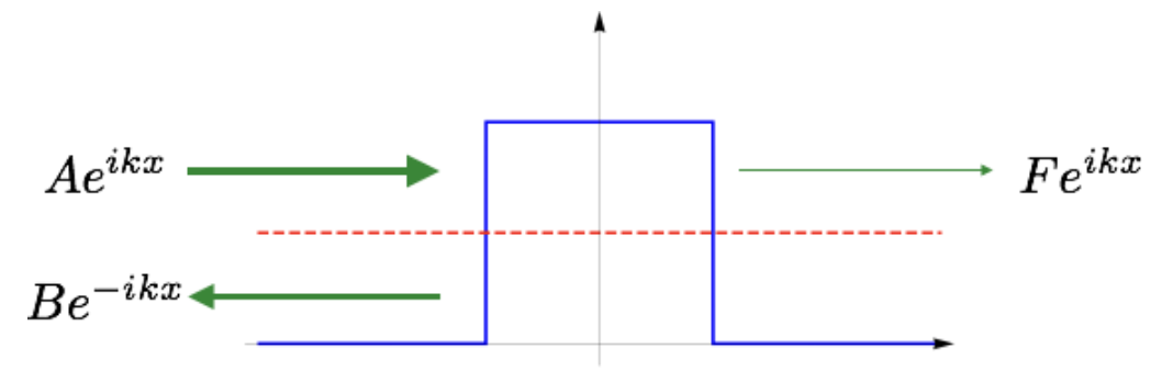
The wave %22%2F%3E%3Cuse%20xlink%3Ahref%3D%22%23b%22%20class%3D%22typst-text%22%20transform%3D%22matrix(1%200%200%20-1%2012.25%2013.732)%22%2F%3E%3Cuse%20xlink%3Ahref%3D%22%23c%22%20class%3D%22typst-text%22%20transform%3D%22matrix(1%200%200%20-1%2019.24%208.287)%22%2F%3E%3Cuse%20xlink%3Ahref%3D%22%23d%22%20class%3D%22typst-text%22%20transform%3D%22matrix(1%200%200%20-1%2023.482%208.287)%22%2F%3E%3Cuse%20xlink%3Ahref%3D%22%23e%22%20class%3D%22typst-text%22%20transform%3D%22matrix(1%200%200%20-1%2029.856%208.287)%22%2F%3E%3C%2Fg%3E%3C%2Fg%3E%3Cdefs%3E%3Csymbol%20id%3D%22a%22%20overflow%3D%22visible%22%3E%3Cpath%20d%3D%22M2.055.045C2.325.045%203.255%200%203.54%200c.225%200%20.33.12.33.345%200%20.135-.09.225-.285.24-.435.015-.645.165-.645.45%200%20.135.135.435.42.885.405.675.69%201.17.885%201.5H7.89c0-.105.015-.315.06-.645.105-1.095.165-1.695.165-1.77%200-.285-.33-.42-1.005-.42-.285%200-.42-.12-.42-.36Q6.69%200%206.96%200c.36%200%201.5.045%201.86.045.3%200%201.365-.045%201.665-.045.225%200%20.33.12.33.36q0%20.225-.405.225c-.42%200-.675.03-.75.075s-.135.18-.15.405l-.9%209.27c-.045.285-.03.405-.345.405-.18%200-.33-.09-.435-.285L2.67%201.8C2.22%201.05%201.62.645.885.585Q.525.563.525.225C.525.075.615%200%20.78%200c.24%200%201.035.045%201.275.045m5.325%208.61.45-4.65H4.605Z%22%2F%3E%3C%2Fsymbol%3E%3Csymbol%20id%3D%22b%22%20overflow%3D%22visible%22%3E%3Cpath%20d%3D%22M1.86%201.935c0%20.36.075.855.225%201.47h.735c.975%200%201.725.12%202.265.345.495.21.825.51.99.885.105.255.15.495.15.69%200%20.825-.78%201.305-1.62%201.305q-.877%200-1.755-.45C1.695%205.58.69%204.215.69%202.565c0-1.53.885-2.73%202.37-2.73.795%200%201.5.195%202.115.57Q5.94.878%206.3%201.35c.105.135.15.24.15.285%200%20.165-.075.255-.24.255-.075%200-.15-.06-.24-.18C5.475%201.05%204.86.63%204.155.45%203.69.33%203.345.27%203.09.27c-.855%200-1.23.81-1.23%201.665m3.765%203.39c0-.99-.96-1.485-2.895-1.485h-.525c.285.99.705%201.65%201.275%201.965.45.255.825.39%201.125.39.54%200%201.02-.33%201.02-.87%22%2F%3E%3C%2Fsymbol%3E%3Csymbol%20id%3D%22c%22%20overflow%3D%22visible%22%3E%3Cpath%20d%3D%22M3.413%206.52a.44.44%200%200%201-.452.441c-.315%200-.62-.293-.62-.609%200-.252.2-.44.452-.44.315%200%20.62.293.62.608M2.016%204.662q-.74%200-1.165-.756c-.242-.42-.357-.714-.357-.882%200-.115.073-.168.21-.168q.17%200%20.23.189c.242.83.588%201.239%201.05%201.239.147%200%20.221-.105.221-.325%200-.137-.105-.473-.315-1.019l-.651-1.67a1.3%201.3%200%200%201-.095-.45c0-.546.473-.924%201.019-.924.493%200%20.872.252%201.155.767.241.42.357.703.357.86%200%20.116-.073.179-.21.179-.063-.01-.136-.063-.21-.168a.1.1%200%200%201-.021-.042C2.993.682%202.646.273%202.194.273q-.22%200-.22.315c0%20.157.052.378.168.651l.83%202.153q.063.172.063.346c0%20.546-.473.924-1.019.924%22%2F%3E%3C%2Fsymbol%3E%3Csymbol%20id%3D%22d%22%20overflow%3D%22visible%22%3E%3Cpath%20d%3D%22M5.954%203.896c0%20.462-.378.766-.84.766-.473%200-1.03-.304-1.68-.924-.473-.451-.851-.745-1.114-.872L3.33%206.92c.01.02.02.083.041.178%200%20.126-.073.189-.21.189l-1.323-.105c-.178-.01-.262-.105-.262-.284%200-.115.105-.178.305-.178.178%200%20.462%200%20.462-.115a.8.8%200%200%200-.042-.221C1.795%204.378%201.313%202.352.798.357.788.315.788.283.788.273c0-.252.125-.378.388-.378.262%200%20.43.157.515.462.167.64.409%201.596.504%201.985.829-.095%201.249-.358%201.249-.809%200-.095-.063-.43-.063-.525%200-.651.494-1.113%201.134-1.113.378%200%20.693.189.934.567.221.347.357.693.42%201.06%200%20.116-.073.179-.21.179a.24.24%200%200%201-.136-.032.8.8%200%200%201-.105-.252C5.208.652%204.914.274%204.546.274c-.21%200-.315.168-.315.493%200%20.126.022.274.053.452.032.115.053.22.053.336%200%20.452-.232.767-.704.924a4%204%200%200%201-.882.21c.2.136.451.346.756.62.493.44.956.976%201.596.976.115%200%20.2-.021.263-.063-.326-.084-.494-.284-.494-.609%200-.252.2-.43.452-.43.378%200%20.63.336.63.714%22%2F%3E%3C%2Fsymbol%3E%3Csymbol%20id%3D%22e%22%20overflow%3D%22visible%22%3E%3Cpath%20d%3D%22M6.122%203.833c0%20.535-.546.797-1.114.797-.472%200-.86-.23-1.154-.692-.252.461-.672.692-1.25.692-.389%200-.798-.167-1.207-.514-.431-.357-.652-.724-.652-1.102%200-.116.074-.179.21-.179.116%200%20.19.063.242.2.189.567.703%201.228%201.375%201.228.389%200%20.578-.21.578-.64%200-.137-.074-.494-.21-1.072l-.357-1.406C2.488.745%202.1.262%201.648.262a.9.9%200%200%200-.461.105c.21.095.398.326.398.567%200%20.253-.199.431-.451.431-.357%200-.63-.315-.63-.672%200-.525.557-.798%201.123-.798.483%200%20.872.231%201.156.693.252-.462.661-.693%201.238-.693.578%200%201.04.231%201.397.693.305.41.462.725.462.924%200%20.115-.063.178-.2.178-.115%200-.199-.073-.241-.21C5.261.924%204.725.263%204.064.263c-.389%200-.589.21-.589.63%200%20.157.179.944.536%202.341.178.682.494%201.029.966%201.029l.095-.01a.9.9%200%200%200%20.367-.085c-.263-.115-.388-.304-.388-.577%200-.252.199-.43.451-.43.357%200%20.62.314.62.672%22%2F%3E%3C%2Fsymbol%3E%3C%2Fdefs%3E%3C%2Fsvg%3E) can be interpreted as the wave go toward the barrier, and the wave
can be interpreted as the wave go toward the barrier, and the wave %22%2F%3E%3Cuse%20xlink%3Ahref%3D%22%23b%22%20class%3D%22typst-text%22%20transform%3D%22matrix(1%200%200%20-1%2012.76%2013.732)%22%2F%3E%3Cuse%20xlink%3Ahref%3D%22%23c%22%20class%3D%22typst-text%22%20transform%3D%22matrix(1%200%200%20-1%2019.75%208.287)%22%2F%3E%3Cuse%20xlink%3Ahref%3D%22%23d%22%20class%3D%22typst-text%22%20transform%3D%22matrix(1%200%200%20-1%2027.919%208.287)%22%2F%3E%3Cuse%20xlink%3Ahref%3D%22%23e%22%20class%3D%22typst-text%22%20transform%3D%22matrix(1%200%200%20-1%2032.161%208.287)%22%2F%3E%3Cuse%20xlink%3Ahref%3D%22%23f%22%20class%3D%22typst-text%22%20transform%3D%22matrix(1%200%200%20-1%2038.534%208.287)%22%2F%3E%3C%2Fg%3E%3C%2Fg%3E%3Cdefs%3E%3Csymbol%20id%3D%22a%22%20overflow%3D%22visible%22%3E%3Cpath%20d%3D%22M11.34%208.145c0%201.365-1.35%202.1-2.82%202.1H3.54c-.345%200-.495-.015-.495-.36%200-.24.3-.225.48-.225.45-.015.72-.045.795-.06s.105-.06.105-.135c0-.03-.015-.12-.06-.27L2.385%201.23C2.31.9%202.16.705%201.935.63%201.83.6%201.56.585%201.095.585.78.585.63.465.63.225.63.075.78%200%201.095%200H6.39c.975%200%201.875.3%202.73.885.945.645%201.425%201.44%201.425%202.37%200%201.185-.975%201.905-2.04%202.115%201.32.315%202.835%201.32%202.835%202.775M8.31%209.66c1.035%200%201.56-.48%201.56-1.455%200-.765-.3-1.395-.93-1.905a3.25%203.25%200%200%200-2.1-.75H4.755l.9%203.6c.12.51.12.51.75.51Zm.42-5.175c.21-.345.315-.69.315-1.065%200-.78-.3-1.455-.915-2.01S6.825.585%206.03.585H4.005c-.15%200-.255%200-.315.015-.09%200-.135.03-.135.075%200%20.015%200%20.06.015.12A748%20748%200%200%200%204.635%205.1h2.76c.645%200%201.08-.21%201.335-.615%22%2F%3E%3C%2Fsymbol%3E%3Csymbol%20id%3D%22b%22%20overflow%3D%22visible%22%3E%3Cpath%20d%3D%22M1.86%201.935c0%20.36.075.855.225%201.47h.735c.975%200%201.725.12%202.265.345.495.21.825.51.99.885.105.255.15.495.15.69%200%20.825-.78%201.305-1.62%201.305q-.877%200-1.755-.45C1.695%205.58.69%204.215.69%202.565c0-1.53.885-2.73%202.37-2.73.795%200%201.5.195%202.115.57Q5.94.878%206.3%201.35c.105.135.15.24.15.285%200%20.165-.075.255-.24.255-.075%200-.15-.06-.24-.18C5.475%201.05%204.86.63%204.155.45%203.69.33%203.345.27%203.09.27c-.855%200-1.23.81-1.23%201.665m3.765%203.39c0-.99-.96-1.485-2.895-1.485h-.525c.285.99.705%201.65%201.275%201.965.45.255.825.39%201.125.39.54%200%201.02-.33%201.02-.87%22%2F%3E%3C%2Fsymbol%3E%3Csymbol%20id%3D%22c%22%20overflow%3D%22visible%22%3E%3Cpath%20d%3D%22M7.308%202.867H.861c-.21%200-.273-.106-.273-.242%200-.137.063-.242.273-.242h6.447c.21%200%20.273.105.273.242%200%20.126-.063.241-.273.241%22%2F%3E%3C%2Fsymbol%3E%3Csymbol%20id%3D%22d%22%20overflow%3D%22visible%22%3E%3Cpath%20d%3D%22M3.413%206.52a.44.44%200%200%201-.452.441c-.315%200-.62-.293-.62-.609%200-.252.2-.44.452-.44.315%200%20.62.293.62.608M2.016%204.662q-.74%200-1.165-.756c-.242-.42-.357-.714-.357-.882%200-.115.073-.168.21-.168q.17%200%20.23.189c.242.83.588%201.239%201.05%201.239.147%200%20.221-.105.221-.325%200-.137-.105-.473-.315-1.019l-.651-1.67a1.3%201.3%200%200%201-.095-.45c0-.546.473-.924%201.019-.924.493%200%20.872.252%201.155.767.241.42.357.703.357.86%200%20.116-.073.179-.21.179-.063-.01-.136-.063-.21-.168a.1.1%200%200%201-.021-.042C2.993.682%202.646.273%202.194.273q-.22%200-.22.315c0%20.157.052.378.168.651l.83%202.153q.063.172.063.346c0%20.546-.473.924-1.019.924%22%2F%3E%3C%2Fsymbol%3E%3Csymbol%20id%3D%22e%22%20overflow%3D%22visible%22%3E%3Cpath%20d%3D%22M5.954%203.896c0%20.462-.378.766-.84.766-.473%200-1.03-.304-1.68-.924-.473-.451-.851-.745-1.114-.872L3.33%206.92c.01.02.02.083.041.178%200%20.126-.073.189-.21.189l-1.323-.105c-.178-.01-.262-.105-.262-.284%200-.115.105-.178.305-.178.178%200%20.462%200%20.462-.115a.8.8%200%200%200-.042-.221C1.795%204.378%201.313%202.352.798.357.788.315.788.283.788.273c0-.252.125-.378.388-.378.262%200%20.43.157.515.462.167.64.409%201.596.504%201.985.829-.095%201.249-.358%201.249-.809%200-.095-.063-.43-.063-.525%200-.651.494-1.113%201.134-1.113.378%200%20.693.189.934.567.221.347.357.693.42%201.06%200%20.116-.073.179-.21.179a.24.24%200%200%201-.136-.032.8.8%200%200%201-.105-.252C5.208.652%204.914.274%204.546.274c-.21%200-.315.168-.315.493%200%20.126.022.274.053.452.032.115.053.22.053.336%200%20.452-.232.767-.704.924a4%204%200%200%201-.882.21c.2.136.451.346.756.62.493.44.956.976%201.596.976.115%200%20.2-.021.263-.063-.326-.084-.494-.284-.494-.609%200-.252.2-.43.452-.43.378%200%20.63.336.63.714%22%2F%3E%3C%2Fsymbol%3E%3Csymbol%20id%3D%22f%22%20overflow%3D%22visible%22%3E%3Cpath%20d%3D%22M6.122%203.833c0%20.535-.546.797-1.114.797-.472%200-.86-.23-1.154-.692-.252.461-.672.692-1.25.692-.389%200-.798-.167-1.207-.514-.431-.357-.652-.724-.652-1.102%200-.116.074-.179.21-.179.116%200%20.19.063.242.2.189.567.703%201.228%201.375%201.228.389%200%20.578-.21.578-.64%200-.137-.074-.494-.21-1.072l-.357-1.406C2.488.745%202.1.262%201.648.262a.9.9%200%200%200-.461.105c.21.095.398.326.398.567%200%20.253-.199.431-.451.431-.357%200-.63-.315-.63-.672%200-.525.557-.798%201.123-.798.483%200%20.872.231%201.156.693.252-.462.661-.693%201.238-.693.578%200%201.04.231%201.397.693.305.41.462.725.462.924%200%20.115-.063.178-.2.178-.115%200-.199-.073-.241-.21C5.261.924%204.725.263%204.064.263c-.389%200-.589.21-.589.63%200%20.157.179.944.536%202.341.178.682.494%201.029.966%201.029l.095-.01a.9.9%200%200%200%20.367-.085c-.263-.115-.388-.304-.388-.577%200-.252.199-.43.451-.43.357%200%20.62.314.62.672%22%2F%3E%3C%2Fsymbol%3E%3C%2Fdefs%3E%3C%2Fsvg%3E) can be interpreted as the wave being reflected by the barrier and wave
can be interpreted as the wave being reflected by the barrier and wave %22%2F%3E%3Cuse%20xlink%3Ahref%3D%22%23b%22%20class%3D%22typst-text%22%20transform%3D%22matrix(1%200%200%20-1%2012.655%2013.732)%22%2F%3E%3Cuse%20xlink%3Ahref%3D%22%23c%22%20class%3D%22typst-text%22%20transform%3D%22matrix(1%200%200%20-1%2019.645%208.287)%22%2F%3E%3Cuse%20xlink%3Ahref%3D%22%23d%22%20class%3D%22typst-text%22%20transform%3D%22matrix(1%200%200%20-1%2023.887%208.287)%22%2F%3E%3Cuse%20xlink%3Ahref%3D%22%23e%22%20class%3D%22typst-text%22%20transform%3D%22matrix(1%200%200%20-1%2030.26%208.287)%22%2F%3E%3C%2Fg%3E%3C%2Fg%3E%3Cdefs%3E%3Csymbol%20id%3D%22a%22%20overflow%3D%22visible%22%3E%3Cpath%20d%3D%22M2.985%209.84c0-.15.165-.225.48-.225.6%200%20.9-.06.9-.195%200-.045-.03-.15-.075-.345L2.34%201.23C2.25.9%202.1.705%201.89.63%201.785.6%201.515.585%201.05.585.72.585.57.555.57.24.57.075.66%200%20.855%200l1.95.045L5.025%200c.24%200%20.36.12.36.345%200%20.255-.165.24-.555.24-.66%200-1.035.03-1.125.105-.045.015-.06.075-.06.15l.96%203.975H6c.69%200%201.17-.03%201.17-.6%200-.195-.03-.435-.105-.72a3%203%200%200%201-.045-.165c0-.165.075-.24.24-.24.075.015.18.12.285.345l.81%203.225c.03.12.045.21.045.255-.045.135-.135.21-.24.21-.12%200-.21-.12-.27-.345-.15-.57-.36-.93-.6-1.11q-.36-.27-1.26-.27H4.755l.93%203.69c.12.51.12.525.75.525h1.95c1.455%200%202.115-.225%202.115-1.56%200-.3-.015-.57-.045-.795-.015-.165-.03-.255-.03-.27%200-.165.075-.24.225-.24s.24.135.27.42l.3%202.565c.045.42-.06.465-.465.465h-7.26c-.345%200-.51-.015-.51-.36%22%2F%3E%3C%2Fsymbol%3E%3Csymbol%20id%3D%22b%22%20overflow%3D%22visible%22%3E%3Cpath%20d%3D%22M1.86%201.935c0%20.36.075.855.225%201.47h.735c.975%200%201.725.12%202.265.345.495.21.825.51.99.885.105.255.15.495.15.69%200%20.825-.78%201.305-1.62%201.305q-.877%200-1.755-.45C1.695%205.58.69%204.215.69%202.565c0-1.53.885-2.73%202.37-2.73.795%200%201.5.195%202.115.57Q5.94.878%206.3%201.35c.105.135.15.24.15.285%200%20.165-.075.255-.24.255-.075%200-.15-.06-.24-.18C5.475%201.05%204.86.63%204.155.45%203.69.33%203.345.27%203.09.27c-.855%200-1.23.81-1.23%201.665m3.765%203.39c0-.99-.96-1.485-2.895-1.485h-.525c.285.99.705%201.65%201.275%201.965.45.255.825.39%201.125.39.54%200%201.02-.33%201.02-.87%22%2F%3E%3C%2Fsymbol%3E%3Csymbol%20id%3D%22c%22%20overflow%3D%22visible%22%3E%3Cpath%20d%3D%22M3.413%206.52a.44.44%200%200%201-.452.441c-.315%200-.62-.293-.62-.609%200-.252.2-.44.452-.44.315%200%20.62.293.62.608M2.016%204.662q-.74%200-1.165-.756c-.242-.42-.357-.714-.357-.882%200-.115.073-.168.21-.168q.17%200%20.23.189c.242.83.588%201.239%201.05%201.239.147%200%20.221-.105.221-.325%200-.137-.105-.473-.315-1.019l-.651-1.67a1.3%201.3%200%200%201-.095-.45c0-.546.473-.924%201.019-.924.493%200%20.872.252%201.155.767.241.42.357.703.357.86%200%20.116-.073.179-.21.179-.063-.01-.136-.063-.21-.168a.1.1%200%200%201-.021-.042C2.993.682%202.646.273%202.194.273q-.22%200-.22.315c0%20.157.052.378.168.651l.83%202.153q.063.172.063.346c0%20.546-.473.924-1.019.924%22%2F%3E%3C%2Fsymbol%3E%3Csymbol%20id%3D%22d%22%20overflow%3D%22visible%22%3E%3Cpath%20d%3D%22M5.954%203.896c0%20.462-.378.766-.84.766-.473%200-1.03-.304-1.68-.924-.473-.451-.851-.745-1.114-.872L3.33%206.92c.01.02.02.083.041.178%200%20.126-.073.189-.21.189l-1.323-.105c-.178-.01-.262-.105-.262-.284%200-.115.105-.178.305-.178.178%200%20.462%200%20.462-.115a.8.8%200%200%200-.042-.221C1.795%204.378%201.313%202.352.798.357.788.315.788.283.788.273c0-.252.125-.378.388-.378.262%200%20.43.157.515.462.167.64.409%201.596.504%201.985.829-.095%201.249-.358%201.249-.809%200-.095-.063-.43-.063-.525%200-.651.494-1.113%201.134-1.113.378%200%20.693.189.934.567.221.347.357.693.42%201.06%200%20.116-.073.179-.21.179a.24.24%200%200%201-.136-.032.8.8%200%200%201-.105-.252C5.208.652%204.914.274%204.546.274c-.21%200-.315.168-.315.493%200%20.126.022.274.053.452.032.115.053.22.053.336%200%20.452-.232.767-.704.924a4%204%200%200%201-.882.21c.2.136.451.346.756.62.493.44.956.976%201.596.976.115%200%20.2-.021.263-.063-.326-.084-.494-.284-.494-.609%200-.252.2-.43.452-.43.378%200%20.63.336.63.714%22%2F%3E%3C%2Fsymbol%3E%3Csymbol%20id%3D%22e%22%20overflow%3D%22visible%22%3E%3Cpath%20d%3D%22M6.122%203.833c0%20.535-.546.797-1.114.797-.472%200-.86-.23-1.154-.692-.252.461-.672.692-1.25.692-.389%200-.798-.167-1.207-.514-.431-.357-.652-.724-.652-1.102%200-.116.074-.179.21-.179.116%200%20.19.063.242.2.189.567.703%201.228%201.375%201.228.389%200%20.578-.21.578-.64%200-.137-.074-.494-.21-1.072l-.357-1.406C2.488.745%202.1.262%201.648.262a.9.9%200%200%200-.461.105c.21.095.398.326.398.567%200%20.253-.199.431-.451.431-.357%200-.63-.315-.63-.672%200-.525.557-.798%201.123-.798.483%200%20.872.231%201.156.693.252-.462.661-.693%201.238-.693.578%200%201.04.231%201.397.693.305.41.462.725.462.924%200%20.115-.063.178-.2.178-.115%200-.199-.073-.241-.21C5.261.924%204.725.263%204.064.263c-.389%200-.589.21-.589.63%200%20.157.179.944.536%202.341.178.682.494%201.029.966%201.029l.095-.01a.9.9%200%200%200%20.367-.085c-.263-.115-.388-.304-.388-.577%200-.252.199-.43.451-.43.357%200%20.62.314.62.672%22%2F%3E%3C%2Fsymbol%3E%3C%2Fdefs%3E%3C%2Fsvg%3E) can be interpreted as the wave go through the barrier.
can be interpreted as the wave go through the barrier.
As there is no probability for the particle to be in region II, the probability current must be same at the point %22%2F%3E%3Cuse%20xlink%3Ahref%3D%22%23b%22%20class%3D%22typst-text%22%20transform%3D%22matrix(1%200%200%20-1%2013.747%207.63)%22%2F%3E%3Cuse%20xlink%3Ahref%3D%22%23c%22%20class%3D%22typst-text%22%20transform%3D%22matrix(1%200%200%20-1%2029.583%207.63)%22%2F%3E%3C%2Fg%3E%3C%2Fg%3E%3Cdefs%3E%3Csymbol%20id%3D%22a%22%20overflow%3D%22visible%22%3E%3Cpath%20d%3D%22M7.905%205.595c0%20.69-.675%201.035-1.425%201.035-.645%200-1.155-.345-1.545-1.035-.315.69-.84%201.035-1.605%201.035-.735%200-1.335-.345-1.815-1.02C1.11%205.025.9%204.59.9%204.305c0-.135.075-.21.225-.21.135%200%20.225.075.255.21.285.87.915%201.89%201.92%201.89.495%200%20.735-.315.735-.93%200-.315-.27-1.485-.795-3.495C2.985.765%202.535.27%201.89.27c-.21%200-.405.045-.57.12q.585.225.585.81c0%20.39-.195.585-.6.585-.495%200-.87-.42-.87-.915%200-.69.705-1.035%201.44-1.035.63%200%201.14.345%201.545%201.035.285-.69.825-1.035%201.605-1.035.72%200%201.32.345%201.8%201.02.405.585.615%201.02.615%201.305%200%20.135-.075.21-.225.21-.135%200-.21-.075-.255-.21C6.705%201.305%206.03.27%205.055.27c-.495%200-.75.3-.75.915%200%20.195.075.615.24%201.29l.51%202.025c.285%201.125.75%201.695%201.41%201.695.21%200%20.405-.045.57-.12-.405-.135-.6-.405-.6-.81%200-.39.21-.585.615-.585.48%200%20.855.435.855.915%22%2F%3E%3C%2Fsymbol%3E%3Csymbol%20id%3D%22b%22%20overflow%3D%22visible%22%3E%3Cpath%20d%3D%22M10.47%205.505H1.2c-.24%200-.36-.12-.36-.345s.12-.345.36-.345h9.27c.24%200%20.36.12.36.345%200%20.18-.165.345-.36.345m0-2.82H1.2c-.24%200-.36-.12-.36-.345s.12-.345.36-.345h9.27c.24%200%20.36.12.36.345a.35.35%200%200%201-.36.345%22%2F%3E%3C%2Fsymbol%3E%3Csymbol%20id%3D%22c%22%20overflow%3D%22visible%22%3E%3Cpath%20d%3D%22M7.47%202.16c0%20.135-.075.21-.24.21-.12%200-.21-.105-.255-.315C6.675.87%206.315.27%205.91.27c-.255%200-.39.21-.39.63%200%20.195.06.555.195%201.08l.855%203.375c.075.285.105.45.105.525q0%20.45-.495.45c-.315%200-.525-.18-.63-.525-.315.555-.765.825-1.335.825-.975%200-1.83-.495-2.58-1.485C.945%204.215.6%203.255.6%202.25.6.945%201.365-.165%202.625-.165%203.27-.165%203.9.18%204.5.87A1.416%201.416%200%200%201%205.88-.165c1.035%200%201.35%201.215%201.59%202.325M5.115%205.61c.135-.315.21-.525.21-.66%200-.06-.015-.135-.03-.24L4.56%201.83a1.7%201.7%200%200%200-.285-.525Q3.443.27%202.655.27c-.585%200-.885.45-.885%201.335q0%20.54.27%201.62c.315%201.275.765%202.13%201.32%202.595.3.255.585.375.87.375.405%200%20.705-.195.885-.585%22%2F%3E%3C%2Fsymbol%3E%3C%2Fdefs%3E%3C%2Fsvg%3E) and
and %22%2F%3E%3Cuse%20xlink%3Ahref%3D%22%23b%22%20class%3D%22typst-text%22%20transform%3D%22matrix(1%200%200%20-1%2013.747%207.63)%22%2F%3E%3Cuse%20xlink%3Ahref%3D%22%23c%22%20class%3D%22typst-text%22%20transform%3D%22matrix(1%200%200%20-1%2029.583%207.63)%22%2F%3E%3Cuse%20xlink%3Ahref%3D%22%23d%22%20class%3D%22typst-text%22%20transform%3D%22matrix(1%200%200%20-1%2041.253%207.63)%22%2F%3E%3C%2Fg%3E%3C%2Fg%3E%3Cdefs%3E%3Csymbol%20id%3D%22a%22%20overflow%3D%22visible%22%3E%3Cpath%20d%3D%22M7.905%205.595c0%20.69-.675%201.035-1.425%201.035-.645%200-1.155-.345-1.545-1.035-.315.69-.84%201.035-1.605%201.035-.735%200-1.335-.345-1.815-1.02C1.11%205.025.9%204.59.9%204.305c0-.135.075-.21.225-.21.135%200%20.225.075.255.21.285.87.915%201.89%201.92%201.89.495%200%20.735-.315.735-.93%200-.315-.27-1.485-.795-3.495C2.985.765%202.535.27%201.89.27c-.21%200-.405.045-.57.12q.585.225.585.81c0%20.39-.195.585-.6.585-.495%200-.87-.42-.87-.915%200-.69.705-1.035%201.44-1.035.63%200%201.14.345%201.545%201.035.285-.69.825-1.035%201.605-1.035.72%200%201.32.345%201.8%201.02.405.585.615%201.02.615%201.305%200%20.135-.075.21-.225.21-.135%200-.21-.075-.255-.21C6.705%201.305%206.03.27%205.055.27c-.495%200-.75.3-.75.915%200%20.195.075.615.24%201.29l.51%202.025c.285%201.125.75%201.695%201.41%201.695.21%200%20.405-.045.57-.12-.405-.135-.6-.405-.6-.81%200-.39.21-.585.615-.585.48%200%20.855.435.855.915%22%2F%3E%3C%2Fsymbol%3E%3Csymbol%20id%3D%22b%22%20overflow%3D%22visible%22%3E%3Cpath%20d%3D%22M10.47%205.505H1.2c-.24%200-.36-.12-.36-.345s.12-.345.36-.345h9.27c.24%200%20.36.12.36.345%200%20.18-.165.345-.36.345m0-2.82H1.2c-.24%200-.36-.12-.36-.345s.12-.345.36-.345h9.27c.24%200%20.36.12.36.345a.35.35%200%200%201-.36.345%22%2F%3E%3C%2Fsymbol%3E%3Csymbol%20id%3D%22c%22%20overflow%3D%22visible%22%3E%3Cpath%20d%3D%22M10.47%204.05H1.2c-.24%200-.36-.105-.36-.3s.12-.3.36-.3h9.27c.24%200%20.36.105.36.3%200%20.18-.18.3-.36.3%22%2F%3E%3C%2Fsymbol%3E%3Csymbol%20id%3D%22d%22%20overflow%3D%22visible%22%3E%3Cpath%20d%3D%22M7.47%202.16c0%20.135-.075.21-.24.21-.12%200-.21-.105-.255-.315C6.675.87%206.315.27%205.91.27c-.255%200-.39.21-.39.63%200%20.195.06.555.195%201.08l.855%203.375c.075.285.105.45.105.525q0%20.45-.495.45c-.315%200-.525-.18-.63-.525-.315.555-.765.825-1.335.825-.975%200-1.83-.495-2.58-1.485C.945%204.215.6%203.255.6%202.25.6.945%201.365-.165%202.625-.165%203.27-.165%203.9.18%204.5.87A1.416%201.416%200%200%201%205.88-.165c1.035%200%201.35%201.215%201.59%202.325M5.115%205.61c.135-.315.21-.525.21-.66%200-.06-.015-.135-.03-.24L4.56%201.83a1.7%201.7%200%200%200-.285-.525Q3.443.27%202.655.27c-.585%200-.885.45-.885%201.335q0%20.54.27%201.62c.315%201.275.765%202.13%201.32%202.595.3.255.585.375.87.375.405%200%20.705-.195.885-.585%22%2F%3E%3C%2Fsymbol%3E%3C%2Fdefs%3E%3C%2Fsvg%3E) .
.
In region I:
![J = \frac{\hbar}{2mi}\left[
\psi\frac{-\partial \psi}{\partial x}^* + \psi^*\frac{\partial \psi}{\partial x}
\right] = \frac{\hbar k}{m}(|A|^2 - |B|^2)](/typst_svg/a689cde417b9f976188a6ade13c5b1e09a3de0fd.svg)
In region III:
![J = \frac{\hbar}{2mi}\left[
\psi\frac{-\partial \psi}{\partial x}^* + \psi^*\frac{\partial \psi}{\partial x}
\right] = \frac{\hbar k}{m}|F|^2](/typst_svg/32b9cbaa8dfcf1aa92a304cc78d1c65ec160b7d2.svg)
Thus, we have
%22%2F%3E%3Cuse%20xlink%3Ahref%3D%22%23b%22%20class%3D%22typst-text%22%20transform%3D%22matrix(1%200%200%20-1%2019.15%2022.417)%22%2F%3E%3Cuse%20xlink%3Ahref%3D%22%23a%22%20class%3D%22typst-text%22%20transform%3D%22matrix(1%200%200%20-1%2035.38%2022.417)%22%2F%3E%3Cuse%20xlink%3Ahref%3D%22%23c%22%20class%3D%22typst-text%22%20transform%3D%22matrix(1%200%200%20-1%2039.55%2016.972)%22%2F%3E%3Cuse%20xlink%3Ahref%3D%22%23d%22%20class%3D%22typst-text%22%20transform%3D%22matrix(1%200%200%20-1%2049.698%2022.417)%22%2F%3E%3Cuse%20xlink%3Ahref%3D%22%23a%22%20class%3D%22typst-text%22%20transform%3D%22matrix(1%200%200%20-1%2064.701%2022.417)%22%2F%3E%3Cuse%20xlink%3Ahref%3D%22%23e%22%20class%3D%22typst-text%22%20transform%3D%22matrix(1%200%200%20-1%2073.851%2022.417)%22%2F%3E%3Cuse%20xlink%3Ahref%3D%22%23a%22%20class%3D%22typst-text%22%20transform%3D%22matrix(1%200%200%20-1%2090.591%2022.417)%22%2F%3E%3Cuse%20xlink%3Ahref%3D%22%23c%22%20class%3D%22typst-text%22%20transform%3D%22matrix(1%200%200%20-1%2094.761%2016.972)%22%2F%3E%3Cuse%20xlink%3Ahref%3D%22%23f%22%20class%3D%22typst-text%22%20transform%3D%22matrix(1%200%200%20-1%20105.742%2022.417)%22%2F%3E%3Cuse%20xlink%3Ahref%3D%22%23a%22%20class%3D%22typst-text%22%20transform%3D%22matrix(1%200%200%20-1%20121.579%2022.417)%22%2F%3E%3Cuse%20xlink%3Ahref%3D%22%23g%22%20class%3D%22typst-text%22%20transform%3D%22matrix(1%200%200%20-1%20130.729%2022.417)%22%2F%3E%3Cuse%20xlink%3Ahref%3D%22%23a%22%20class%3D%22typst-text%22%20transform%3D%22matrix(1%200%200%20-1%20147.364%2022.417)%22%2F%3E%3Cuse%20xlink%3Ahref%3D%22%23c%22%20class%3D%22typst-text%22%20transform%3D%22matrix(1%200%200%20-1%20151.534%2016.972)%22%2F%3E%3C%2Fg%3E%3C%2Fg%3E%3Cdefs%3E%3Csymbol%20id%3D%22a%22%20overflow%3D%22visible%22%3E%3Cpath%20d%3D%22M2.085-3.75c.195%200%20.3.12.3.36v14.28c0%20.24-.105.36-.3.36s-.3-.12-.3-.36V-3.39c0-.24.105-.36.3-.36%22%2F%3E%3C%2Fsymbol%3E%3Csymbol%20id%3D%22b%22%20overflow%3D%22visible%22%3E%3Cpath%20d%3D%22M2.055.045C2.325.045%203.255%200%203.54%200c.225%200%20.33.12.33.345%200%20.135-.09.225-.285.24-.435.015-.645.165-.645.45%200%20.135.135.435.42.885.405.675.69%201.17.885%201.5H7.89c0-.105.015-.315.06-.645.105-1.095.165-1.695.165-1.77%200-.285-.33-.42-1.005-.42-.285%200-.42-.12-.42-.36Q6.69%200%206.96%200c.36%200%201.5.045%201.86.045.3%200%201.365-.045%201.665-.045.225%200%20.33.12.33.36q0%20.225-.405.225c-.42%200-.675.03-.75.075s-.135.18-.15.405l-.9%209.27c-.045.285-.03.405-.345.405-.18%200-.33-.09-.435-.285L2.67%201.8C2.22%201.05%201.62.645.885.585Q.525.563.525.225C.525.075.615%200%20.78%200c.24%200%201.035.045%201.275.045m5.325%208.61.45-4.65H4.605Z%22%2F%3E%3C%2Fsymbol%3E%3Csymbol%20id%3D%22c%22%20overflow%3D%22visible%22%3E%3Cpath%20d%3D%22M1.25%204.452c.335%200%20.587.252.587.588%200%20.378-.199.577-.587.588.23.494.756.892%201.438.892.924%200%201.533-.692%201.533-1.616%200-.505-.178-.988-.546-1.46a5%205%200%200%200-.41-.504L.777.473C.64.347.661.315.661%200h4.326l.326%201.974h-.441c-.074-.556-.157-.882-.252-.955-.053-.032-.378-.053-.997-.053H1.837c.704.62%201.355%201.176%201.974%201.67.473.367.809.692%201.019.976q.473.614.473%201.292c0%20.65-.252%201.165-.767%201.543-.451.346-1.018.525-1.69.525a2.36%202.36%200%200%201-1.502-.504c-.452-.367-.683-.83-.683-1.396%200-.357.263-.62.589-.62%22%2F%3E%3C%2Fsymbol%3E%3Csymbol%20id%3D%22d%22%20overflow%3D%22visible%22%3E%3Cpath%20d%3D%22M10.47%204.05H1.2c-.24%200-.36-.105-.36-.3s.12-.3.36-.3h9.27c.24%200%20.36.105.36.3%200%20.18-.18.3-.36.3%22%2F%3E%3C%2Fsymbol%3E%3Csymbol%20id%3D%22e%22%20overflow%3D%22visible%22%3E%3Cpath%20d%3D%22M11.34%208.145c0%201.365-1.35%202.1-2.82%202.1H3.54c-.345%200-.495-.015-.495-.36%200-.24.3-.225.48-.225.45-.015.72-.045.795-.06s.105-.06.105-.135c0-.03-.015-.12-.06-.27L2.385%201.23C2.31.9%202.16.705%201.935.63%201.83.6%201.56.585%201.095.585.78.585.63.465.63.225.63.075.78%200%201.095%200H6.39c.975%200%201.875.3%202.73.885.945.645%201.425%201.44%201.425%202.37%200%201.185-.975%201.905-2.04%202.115%201.32.315%202.835%201.32%202.835%202.775M8.31%209.66c1.035%200%201.56-.48%201.56-1.455%200-.765-.3-1.395-.93-1.905a3.25%203.25%200%200%200-2.1-.75H4.755l.9%203.6c.12.51.12.51.75.51Zm.42-5.175c.21-.345.315-.69.315-1.065%200-.78-.3-1.455-.915-2.01S6.825.585%206.03.585H4.005c-.15%200-.255%200-.315.015-.09%200-.135.03-.135.075%200%20.015%200%20.06.015.12A748%20748%200%200%200%204.635%205.1h2.76c.645%200%201.08-.21%201.335-.615%22%2F%3E%3C%2Fsymbol%3E%3Csymbol%20id%3D%22f%22%20overflow%3D%22visible%22%3E%3Cpath%20d%3D%22M10.47%205.505H1.2c-.24%200-.36-.12-.36-.345s.12-.345.36-.345h9.27c.24%200%20.36.12.36.345%200%20.18-.165.345-.36.345m0-2.82H1.2c-.24%200-.36-.12-.36-.345s.12-.345.36-.345h9.27c.24%200%20.36.12.36.345a.35.35%200%200%201-.36.345%22%2F%3E%3C%2Fsymbol%3E%3Csymbol%20id%3D%22g%22%20overflow%3D%22visible%22%3E%3Cpath%20d%3D%22M2.985%209.84c0-.15.165-.225.48-.225.6%200%20.9-.06.9-.195%200-.045-.03-.15-.075-.345L2.34%201.23C2.25.9%202.1.705%201.89.63%201.785.6%201.515.585%201.05.585.72.585.57.555.57.24.57.075.66%200%20.855%200l1.95.045L5.025%200c.24%200%20.36.12.36.345%200%20.255-.165.24-.555.24-.66%200-1.035.03-1.125.105-.045.015-.06.075-.06.15l.96%203.975H6c.69%200%201.17-.03%201.17-.6%200-.195-.03-.435-.105-.72a3%203%200%200%201-.045-.165c0-.165.075-.24.24-.24.075.015.18.12.285.345l.81%203.225c.03.12.045.21.045.255-.045.135-.135.21-.24.21-.12%200-.21-.12-.27-.345-.15-.57-.36-.93-.6-1.11q-.36-.27-1.26-.27H4.755l.93%203.69c.12.51.12.525.75.525h1.95c1.455%200%202.115-.225%202.115-1.56%200-.3-.015-.57-.045-.795-.015-.165-.03-.255-.03-.27%200-.165.075-.24.225-.24s.24.135.27.42l.3%202.565c.045.42-.06.465-.465.465h-7.26c-.345%200-.51-.015-.51-.36%22%2F%3E%3C%2Fsymbol%3E%3C%2Fdefs%3E%3C%2Fsvg%3E)
We define the reflection probability %22%2F%3E%3C%2Fg%3E%3C%2Fg%3E%3Cdefs%3E%3Csymbol%20id%3D%22a%22%20overflow%3D%22visible%22%3E%3Cpath%20d%3D%22M11.085%207.965c0%20.765-.39%201.35-1.155%201.77-.615.345-1.35.51-2.175.51h-4.23c-.345%200-.495-.015-.495-.36%200-.105.045-.18.135-.195.15-.015.27-.03.345-.03.45-.015.705-.045.78-.06s.12-.06.12-.135c0-.03-.015-.12-.06-.27L2.37%201.23C2.295.9%202.145.69%201.92.615%201.815.585%201.545.57%201.08.57.75.57.615.555.615.225q0-.247.27-.225l1.86.045L4.635%200c.24-.015.36.12.36.345%200%20.15-.165.225-.48.225-.6%200-.9.075-.9.21%200%200%20.015.03.045.24l.96%203.885h1.725c1.035%200%201.56-.435%201.56-1.29%200-.135-.075-.465-.21-1.005-.165-.63-.24-1.05-.24-1.275C7.455.195%208.34-.33%209.48-.33c.42%200%20.825.195%201.23.57s.615.78.615%201.2c0%20.15-.075.225-.24.225-.105%200-.195-.075-.24-.24C10.68.96%2010.47.615%2010.23.42s-.465-.3-.69-.3c-.345%200-.525.285-.525.84%200%20.36.045.915.15%201.68.045.315.06.54.06.705%200%20.795-.42%201.38-1.26%201.74%201.41.345%203.12%201.35%203.12%202.88M9.135%209.24q.45-.293.45-.99c0-.3-.06-.645-.195-1.05q-.607-1.845-3.06-1.845H4.74l.945%203.795q.113.472.36.495c.075.015.375.015.9.015.975%200%201.545-.03%202.19-.42%22%2F%3E%3C%2Fsymbol%3E%3C%2Fdefs%3E%3C%2Fsvg%3E) and transmission probability
and transmission probability %22%2F%3E%3C%2Fg%3E%3C%2Fg%3E%3Cdefs%3E%3Csymbol%20id%3D%22a%22%20overflow%3D%22visible%22%3E%3Cpath%20d%3D%22M5.16%209.465c0-.045-.015-.15-.06-.3l-1.98-7.92c-.06-.225-.12-.36-.165-.42C2.82.66%202.31.585%201.41.585.945.585.735.63.735.24c0-.165.105-.24.3-.24.765%200%201.845.06%202.49.045L4.755.03C4.965.03%205.79%200%206.045%200s.375.12.375.36c0%20.15-.18.225-.555.225-.78%200-1.23.03-1.365.105-.045.03-.075.09-.075.18L6.45%209.045c.045.21.09.345.135.39q.09.135%201.08.135c.825%200%201.395-.06%201.68-.195s.435-.45.435-.96c0-.27-.045-.66-.12-1.17-.03-.12-.045-.21-.045-.285%200-.165.075-.255.24-.255.135%200%20.225.135.27.39l.405%202.58c.015.075.03.165.03.255%200%20.15-.15.225-.465.225h-8.22c-.39%200-.42-.045-.54-.33L.45%207.215a5%205%200%200%201-.09-.285c0-.15.075-.225.24-.225.12%200%20.225.12.3.345.375%201.095.75%201.77%201.095%202.055.39.315%201.14.465%202.235.465h.585c.165%200%20.345.015.345-.105%22%2F%3E%3C%2Fsymbol%3E%3C%2Fdefs%3E%3C%2Fsvg%3E) as
as
%22%2F%3E%3Cuse%20xlink%3Ahref%3D%22%23b%22%20class%3D%22typst-text%22%20transform%3D%22matrix(1%200%200%20-1%2025.912%2028.747)%22%2F%3E%3Cg%20class%3D%22typst-group%22%3E%3Cuse%20xlink%3Ahref%3D%22%23c%22%20class%3D%22typst-text%22%20transform%3D%22matrix(1%200%200%20-1%2043.248%2018.592)%22%2F%3E%3Cuse%20xlink%3Ahref%3D%22%23d%22%20class%3D%22typst-text%22%20transform%3D%22matrix(1%200%200%20-1%2052.398%2018.592)%22%2F%3E%3Cuse%20xlink%3Ahref%3D%22%23c%22%20class%3D%22typst-text%22%20transform%3D%22matrix(1%200%200%20-1%2069.138%2018.592)%22%2F%3E%3Cuse%20xlink%3Ahref%3D%22%23e%22%20class%3D%22typst-text%22%20transform%3D%22matrix(1%200%200%20-1%2073.308%2013.147)%22%2F%3E%3Cuse%20xlink%3Ahref%3D%22%23c%22%20class%3D%22typst-text%22%20transform%3D%22matrix(1%200%200%20-1%2043.503%2039.037)%22%2F%3E%3Cuse%20xlink%3Ahref%3D%22%23f%22%20class%3D%22typst-text%22%20transform%3D%22matrix(1%200%200%20-1%2052.653%2039.037)%22%2F%3E%3Cuse%20xlink%3Ahref%3D%22%23c%22%20class%3D%22typst-text%22%20transform%3D%22matrix(1%200%200%20-1%2068.883%2039.037)%22%2F%3E%3Cuse%20xlink%3Ahref%3D%22%23e%22%20class%3D%22typst-text%22%20transform%3D%22matrix(1%200%200%20-1%2073.053%2034.702)%22%2F%3E%3Cpath%20fill%3D%22none%22%20stroke%3D%22%23000%22%20stroke-width%3D%22.72%22%20d%3D%22M43.248%2024.997h36.875%22%20class%3D%22typst-shape%22%2F%3E%3C%2Fg%3E%3C%2Fg%3E%3Cg%20class%3D%22typst-group%22%3E%3Cuse%20xlink%3Ahref%3D%22%23g%22%20class%3D%22typst-text%22%20transform%3D%22matrix(1%200%200%20-1%2010.765%2075.109)%22%2F%3E%3Cuse%20xlink%3Ahref%3D%22%23b%22%20class%3D%22typst-text%22%20transform%3D%22matrix(1%200%200%20-1%2025.912%2075.109)%22%2F%3E%3Cg%20class%3D%22typst-group%22%3E%3Cuse%20xlink%3Ahref%3D%22%23c%22%20class%3D%22typst-text%22%20transform%3D%22matrix(1%200%200%20-1%2043.248%2064.954)%22%2F%3E%3Cuse%20xlink%3Ahref%3D%22%23h%22%20class%3D%22typst-text%22%20transform%3D%22matrix(1%200%200%20-1%2052.398%2064.954)%22%2F%3E%3Cuse%20xlink%3Ahref%3D%22%23c%22%20class%3D%22typst-text%22%20transform%3D%22matrix(1%200%200%20-1%2069.033%2064.954)%22%2F%3E%3Cuse%20xlink%3Ahref%3D%22%23e%22%20class%3D%22typst-text%22%20transform%3D%22matrix(1%200%200%20-1%2073.203%2059.509)%22%2F%3E%3Cuse%20xlink%3Ahref%3D%22%23c%22%20class%3D%22typst-text%22%20transform%3D%22matrix(1%200%200%20-1%2043.45%2085.399)%22%2F%3E%3Cuse%20xlink%3Ahref%3D%22%23f%22%20class%3D%22typst-text%22%20transform%3D%22matrix(1%200%200%20-1%2052.6%2085.399)%22%2F%3E%3Cuse%20xlink%3Ahref%3D%22%23c%22%20class%3D%22typst-text%22%20transform%3D%22matrix(1%200%200%20-1%2068.83%2085.399)%22%2F%3E%3Cuse%20xlink%3Ahref%3D%22%23e%22%20class%3D%22typst-text%22%20transform%3D%22matrix(1%200%200%20-1%2073%2081.064)%22%2F%3E%3Cpath%20fill%3D%22none%22%20stroke%3D%22%23000%22%20stroke-width%3D%22.72%22%20d%3D%22M43.248%2071.359h36.77%22%20class%3D%22typst-shape%22%2F%3E%3C%2Fg%3E%3C%2Fg%3E%3C%2Fg%3E%3C%2Fg%3E%3C%2Fg%3E%3C%2Fg%3E%3Cdefs%3E%3Csymbol%20id%3D%22a%22%20overflow%3D%22visible%22%3E%3Cpath%20d%3D%22M11.085%207.965c0%20.765-.39%201.35-1.155%201.77-.615.345-1.35.51-2.175.51h-4.23c-.345%200-.495-.015-.495-.36%200-.105.045-.18.135-.195.15-.015.27-.03.345-.03.45-.015.705-.045.78-.06s.12-.06.12-.135c0-.03-.015-.12-.06-.27L2.37%201.23C2.295.9%202.145.69%201.92.615%201.815.585%201.545.57%201.08.57.75.57.615.555.615.225q0-.247.27-.225l1.86.045L4.635%200c.24-.015.36.12.36.345%200%20.15-.165.225-.48.225-.6%200-.9.075-.9.21%200%200%20.015.03.045.24l.96%203.885h1.725c1.035%200%201.56-.435%201.56-1.29%200-.135-.075-.465-.21-1.005-.165-.63-.24-1.05-.24-1.275C7.455.195%208.34-.33%209.48-.33c.42%200%20.825.195%201.23.57s.615.78.615%201.2c0%20.15-.075.225-.24.225-.105%200-.195-.075-.24-.24C10.68.96%2010.47.615%2010.23.42s-.465-.3-.69-.3c-.345%200-.525.285-.525.84%200%20.36.045.915.15%201.68.045.315.06.54.06.705%200%20.795-.42%201.38-1.26%201.74%201.41.345%203.12%201.35%203.12%202.88M9.135%209.24q.45-.293.45-.99c0-.3-.06-.645-.195-1.05q-.607-1.845-3.06-1.845H4.74l.945%203.795q.113.472.36.495c.075.015.375.015.9.015.975%200%201.545-.03%202.19-.42%22%2F%3E%3C%2Fsymbol%3E%3Csymbol%20id%3D%22b%22%20overflow%3D%22visible%22%3E%3Cpath%20d%3D%22M10.47%205.505H1.2c-.24%200-.36-.12-.36-.345s.12-.345.36-.345h9.27c.24%200%20.36.12.36.345%200%20.18-.165.345-.36.345m0-2.82H1.2c-.24%200-.36-.12-.36-.345s.12-.345.36-.345h9.27c.24%200%20.36.12.36.345a.35.35%200%200%201-.36.345%22%2F%3E%3C%2Fsymbol%3E%3Csymbol%20id%3D%22c%22%20overflow%3D%22visible%22%3E%3Cpath%20d%3D%22M2.085-3.75c.195%200%20.3.12.3.36v14.28c0%20.24-.105.36-.3.36s-.3-.12-.3-.36V-3.39c0-.24.105-.36.3-.36%22%2F%3E%3C%2Fsymbol%3E%3Csymbol%20id%3D%22d%22%20overflow%3D%22visible%22%3E%3Cpath%20d%3D%22M11.34%208.145c0%201.365-1.35%202.1-2.82%202.1H3.54c-.345%200-.495-.015-.495-.36%200-.24.3-.225.48-.225.45-.015.72-.045.795-.06s.105-.06.105-.135c0-.03-.015-.12-.06-.27L2.385%201.23C2.31.9%202.16.705%201.935.63%201.83.6%201.56.585%201.095.585.78.585.63.465.63.225.63.075.78%200%201.095%200H6.39c.975%200%201.875.3%202.73.885.945.645%201.425%201.44%201.425%202.37%200%201.185-.975%201.905-2.04%202.115%201.32.315%202.835%201.32%202.835%202.775M8.31%209.66c1.035%200%201.56-.48%201.56-1.455%200-.765-.3-1.395-.93-1.905a3.25%203.25%200%200%200-2.1-.75H4.755l.9%203.6c.12.51.12.51.75.51Zm.42-5.175c.21-.345.315-.69.315-1.065%200-.78-.3-1.455-.915-2.01S6.825.585%206.03.585H4.005c-.15%200-.255%200-.315.015-.09%200-.135.03-.135.075%200%20.015%200%20.06.015.12A748%20748%200%200%200%204.635%205.1h2.76c.645%200%201.08-.21%201.335-.615%22%2F%3E%3C%2Fsymbol%3E%3Csymbol%20id%3D%22e%22%20overflow%3D%22visible%22%3E%3Cpath%20d%3D%22M1.25%204.452c.335%200%20.587.252.587.588%200%20.378-.199.577-.587.588.23.494.756.892%201.438.892.924%200%201.533-.692%201.533-1.616%200-.505-.178-.988-.546-1.46a5%205%200%200%200-.41-.504L.777.473C.64.347.661.315.661%200h4.326l.326%201.974h-.441c-.074-.556-.157-.882-.252-.955-.053-.032-.378-.053-.997-.053H1.837c.704.62%201.355%201.176%201.974%201.67.473.367.809.692%201.019.976q.473.614.473%201.292c0%20.65-.252%201.165-.767%201.543-.451.346-1.018.525-1.69.525a2.36%202.36%200%200%201-1.502-.504c-.452-.367-.683-.83-.683-1.396%200-.357.263-.62.589-.62%22%2F%3E%3C%2Fsymbol%3E%3Csymbol%20id%3D%22f%22%20overflow%3D%22visible%22%3E%3Cpath%20d%3D%22M2.055.045C2.325.045%203.255%200%203.54%200c.225%200%20.33.12.33.345%200%20.135-.09.225-.285.24-.435.015-.645.165-.645.45%200%20.135.135.435.42.885.405.675.69%201.17.885%201.5H7.89c0-.105.015-.315.06-.645.105-1.095.165-1.695.165-1.77%200-.285-.33-.42-1.005-.42-.285%200-.42-.12-.42-.36Q6.69%200%206.96%200c.36%200%201.5.045%201.86.045.3%200%201.365-.045%201.665-.045.225%200%20.33.12.33.36q0%20.225-.405.225c-.42%200-.675.03-.75.075s-.135.18-.15.405l-.9%209.27c-.045.285-.03.405-.345.405-.18%200-.33-.09-.435-.285L2.67%201.8C2.22%201.05%201.62.645.885.585Q.525.563.525.225C.525.075.615%200%20.78%200c.24%200%201.035.045%201.275.045m5.325%208.61.45-4.65H4.605Z%22%2F%3E%3C%2Fsymbol%3E%3Csymbol%20id%3D%22g%22%20overflow%3D%22visible%22%3E%3Cpath%20d%3D%22M5.16%209.465c0-.045-.015-.15-.06-.3l-1.98-7.92c-.06-.225-.12-.36-.165-.42C2.82.66%202.31.585%201.41.585.945.585.735.63.735.24c0-.165.105-.24.3-.24.765%200%201.845.06%202.49.045L4.755.03C4.965.03%205.79%200%206.045%200s.375.12.375.36c0%20.15-.18.225-.555.225-.78%200-1.23.03-1.365.105-.045.03-.075.09-.075.18L6.45%209.045c.045.21.09.345.135.39q.09.135%201.08.135c.825%200%201.395-.06%201.68-.195s.435-.45.435-.96c0-.27-.045-.66-.12-1.17-.03-.12-.045-.21-.045-.285%200-.165.075-.255.24-.255.135%200%20.225.135.27.39l.405%202.58c.015.075.03.165.03.255%200%20.15-.15.225-.465.225h-8.22c-.39%200-.42-.045-.54-.33L.45%207.215a5%205%200%200%201-.09-.285c0-.15.075-.225.24-.225.12%200%20.225.12.3.345.375%201.095.75%201.77%201.095%202.055.39.315%201.14.465%202.235.465h.585c.165%200%20.345.015.345-.105%22%2F%3E%3C%2Fsymbol%3E%3Csymbol%20id%3D%22h%22%20overflow%3D%22visible%22%3E%3Cpath%20d%3D%22M2.985%209.84c0-.15.165-.225.48-.225.6%200%20.9-.06.9-.195%200-.045-.03-.15-.075-.345L2.34%201.23C2.25.9%202.1.705%201.89.63%201.785.6%201.515.585%201.05.585.72.585.57.555.57.24.57.075.66%200%20.855%200l1.95.045L5.025%200c.24%200%20.36.12.36.345%200%20.255-.165.24-.555.24-.66%200-1.035.03-1.125.105-.045.015-.06.075-.06.15l.96%203.975H6c.69%200%201.17-.03%201.17-.6%200-.195-.03-.435-.105-.72a3%203%200%200%201-.045-.165c0-.165.075-.24.24-.24.075.015.18.12.285.345l.81%203.225c.03.12.045.21.045.255-.045.135-.135.21-.24.21-.12%200-.21-.12-.27-.345-.15-.57-.36-.93-.6-1.11q-.36-.27-1.26-.27H4.755l.93%203.69c.12.51.12.525.75.525h1.95c1.455%200%202.115-.225%202.115-1.56%200-.3-.015-.57-.045-.795-.015-.165-.03-.255-.03-.27%200-.165.075-.24.225-.24s.24.135.27.42l.3%202.565c.045.42-.06.465-.465.465h-7.26c-.345%200-.51-.015-.51-.36%22%2F%3E%3C%2Fsymbol%3E%3C%2Fdefs%3E%3C%2Fsvg%3E)
Then, we have
%22%2F%3E%3Cuse%20xlink%3Ahref%3D%22%23b%22%20class%3D%22typst-text%22%20transform%3D%22matrix(1%200%200%20-1%2025.078%2020.245)%22%2F%3E%3Cuse%20xlink%3Ahref%3D%22%23c%22%20class%3D%22typst-text%22%20transform%3D%22matrix(1%200%200%20-1%2040.082%2020.245)%22%2F%3E%3Cuse%20xlink%3Ahref%3D%22%23d%22%20class%3D%22typst-text%22%20transform%3D%22matrix(1%200%200%20-1%2055.228%2020.245)%22%2F%3E%3Cuse%20xlink%3Ahref%3D%22%23e%22%20class%3D%22typst-text%22%20transform%3D%22matrix(1%200%200%20-1%2071.065%2020.245)%22%2F%3E%3C%2Fg%3E%3C%2Fg%3E%3Cdefs%3E%3Csymbol%20id%3D%22a%22%20overflow%3D%22visible%22%3E%3Cpath%20d%3D%22M11.085%207.965c0%20.765-.39%201.35-1.155%201.77-.615.345-1.35.51-2.175.51h-4.23c-.345%200-.495-.015-.495-.36%200-.105.045-.18.135-.195.15-.015.27-.03.345-.03.45-.015.705-.045.78-.06s.12-.06.12-.135c0-.03-.015-.12-.06-.27L2.37%201.23C2.295.9%202.145.69%201.92.615%201.815.585%201.545.57%201.08.57.75.57.615.555.615.225q0-.247.27-.225l1.86.045L4.635%200c.24-.015.36.12.36.345%200%20.15-.165.225-.48.225-.6%200-.9.075-.9.21%200%200%20.015.03.045.24l.96%203.885h1.725c1.035%200%201.56-.435%201.56-1.29%200-.135-.075-.465-.21-1.005-.165-.63-.24-1.05-.24-1.275C7.455.195%208.34-.33%209.48-.33c.42%200%20.825.195%201.23.57s.615.78.615%201.2c0%20.15-.075.225-.24.225-.105%200-.195-.075-.24-.24C10.68.96%2010.47.615%2010.23.42s-.465-.3-.69-.3c-.345%200-.525.285-.525.84%200%20.36.045.915.15%201.68.045.315.06.54.06.705%200%20.795-.42%201.38-1.26%201.74%201.41.345%203.12%201.35%203.12%202.88M9.135%209.24q.45-.293.45-.99c0-.3-.06-.645-.195-1.05q-.607-1.845-3.06-1.845H4.74l.945%203.795q.113.472.36.495c.075.015.375.015.9.015.975%200%201.545-.03%202.19-.42%22%2F%3E%3C%2Fsymbol%3E%3Csymbol%20id%3D%22b%22%20overflow%3D%22visible%22%3E%3Cpath%20d%3D%22M10.47%204.11H6.195v4.275q0%20.36-.36.36t-.36-.36V4.11H1.2q-.36%200-.36-.36t.36-.36h4.275V-.885q0-.36.36-.36t.36.36V3.39h4.275q.36%200%20.36.36c0%20.195-.165.36-.36.36%22%2F%3E%3C%2Fsymbol%3E%3Csymbol%20id%3D%22c%22%20overflow%3D%22visible%22%3E%3Cpath%20d%3D%22M5.16%209.465c0-.045-.015-.15-.06-.3l-1.98-7.92c-.06-.225-.12-.36-.165-.42C2.82.66%202.31.585%201.41.585.945.585.735.63.735.24c0-.165.105-.24.3-.24.765%200%201.845.06%202.49.045L4.755.03C4.965.03%205.79%200%206.045%200s.375.12.375.36c0%20.15-.18.225-.555.225-.78%200-1.23.03-1.365.105-.045.03-.075.09-.075.18L6.45%209.045c.045.21.09.345.135.39q.09.135%201.08.135c.825%200%201.395-.06%201.68-.195s.435-.45.435-.96c0-.27-.045-.66-.12-1.17-.03-.12-.045-.21-.045-.285%200-.165.075-.255.24-.255.135%200%20.225.135.27.39l.405%202.58c.015.075.03.165.03.255%200%20.15-.15.225-.465.225h-8.22c-.39%200-.42-.045-.54-.33L.45%207.215a5%205%200%200%201-.09-.285c0-.15.075-.225.24-.225.12%200%20.225.12.3.345.375%201.095.75%201.77%201.095%202.055.39.315%201.14.465%202.235.465h.585c.165%200%20.345.015.345-.105%22%2F%3E%3C%2Fsymbol%3E%3Csymbol%20id%3D%22d%22%20overflow%3D%22visible%22%3E%3Cpath%20d%3D%22M10.47%205.505H1.2c-.24%200-.36-.12-.36-.345s.12-.345.36-.345h9.27c.24%200%20.36.12.36.345%200%20.18-.165.345-.36.345m0-2.82H1.2c-.24%200-.36-.12-.36-.345s.12-.345.36-.345h9.27c.24%200%20.36.12.36.345a.35.35%200%200%201-.36.345%22%2F%3E%3C%2Fsymbol%3E%3Csymbol%20id%3D%22e%22%20overflow%3D%22visible%22%3E%3Cpath%20d%3D%22M4.035%209.99q-.922-.945-2.7-.945V8.46c.78%200%201.425.12%201.92.36V1.23c0-.27-.06-.45-.195-.525s-.51-.12-1.11-.12h-.525V0q.563.045%202.43.045T6.285%200v.585H5.76c-.615%200-.99.045-1.11.12s-.195.255-.195.525v8.31c0%20.36-.03.45-.42.45%22%2F%3E%3C%2Fsymbol%3E%3C%2Fdefs%3E%3C%2Fsvg%3E)
0.10.2 Quantum Tunnelling through High and Thin Barrier
We consider a barrier that is infinitely high and thin at origin.
To state this formally, we consider the potential to be the limiting behaviour of the Dirac delta function potential.

and
%22%2F%3E%3Cuse%20xlink%3Ahref%3D%22%23b%22%20class%3D%22typst-text%22%20transform%3D%22matrix(1%200%200%20-1%2021.367%2021.22)%22%2F%3E%3Cg%20class%3D%22typst-text%22%20transform%3D%22matrix(1%200%200%20-1%2039.14%2021.22)%22%3E%3Cuse%20xlink%3Ahref%3D%22%23c%22%2F%3E%3Cuse%20xlink%3Ahref%3D%22%23d%22%20x%3D%224.17%22%2F%3E%3Cuse%20xlink%3Ahref%3D%22%23e%22%20x%3D%228.34%22%2F%3E%3C%2Fg%3E%3Cuse%20xlink%3Ahref%3D%22%23f%22%20class%3D%22typst-text%22%20transform%3D%22matrix(1%200%200%20-1%2037.203%2030.896)%22%2F%3E%3Cuse%20xlink%3Ahref%3D%22%23g%22%20class%3D%22typst-text%22%20transform%3D%22matrix(1%200%200%20-1%2045.435%2030.896)%22%2F%3E%3Cuse%20xlink%3Ahref%3D%22%23h%22%20class%3D%22typst-text%22%20transform%3D%22matrix(1%200%200%20-1%2055.935%2030.896)%22%2F%3E%3Cuse%20xlink%3Ahref%3D%22%23a%22%20class%3D%22typst-text%22%20transform%3D%22matrix(1%200%200%20-1%2064.41%2021.22)%22%2F%3E%3Cuse%20xlink%3Ahref%3D%22%23f%22%20class%3D%22typst-text%22%20transform%3D%22matrix(1%200%200%20-1%2071.07%2024.925)%22%2F%3E%3Cuse%20xlink%3Ahref%3D%22%23i%22%20class%3D%22typst-text%22%20transform%3D%22matrix(1%200%200%20-1%2080.142%2021.22)%22%2F%3E%3Cuse%20xlink%3Ahref%3D%22%23j%22%20class%3D%22typst-text%22%20transform%3D%22matrix(1%200%200%20-1%2085.977%2021.22)%22%2F%3E%3Cuse%20xlink%3Ahref%3D%22%23k%22%20class%3D%22typst-text%22%20transform%3D%22matrix(1%200%200%20-1%2094.557%2021.22)%22%2F%3E%3C%2Fg%3E%3C%2Fg%3E%3Cdefs%3E%3Csymbol%20id%3D%22a%22%20overflow%3D%22visible%22%3E%3Cpath%20d%3D%22M6.78%209.96c0%20.225-.12.375-.36.435-.765.195-1.335.285-1.695.285-1.065%200-1.71-.6-1.71-1.59%200-.585.285-1.425.87-2.52C2.34%206.18%201.14%204.815.765%203.3a4%204%200%200%201-.12-.915c0-.57.135-1.08.42-1.515.45-.69%201.11-1.035%201.965-1.035.63%200%201.2.285%201.725.87C5.58%201.65%206%202.85%206%204.275c0%20.915-.3%201.755-.915%202.52l-.105.135c-.975%201.26-1.455%202.1-1.455%202.52%200%20.09.015.165.06.225.15.27.39.405.735.39.255%200%20.57-.12.945-.345.465-.285.75-.42.855-.42.33%200%20.66.27.66.66M1.665%201.965c0%20.855.21%201.68.645%202.49.465.9%201.065%201.47%201.8%201.695.33-.57.555-1.155.69-1.74.045-.225.06-.48.06-.735%200-.42-.045-.81-.135-1.185C4.35%201.02%203.78.285%203.045.285c-.855%200-1.38.705-1.38%201.68%22%2F%3E%3C%2Fsymbol%3E%3Csymbol%20id%3D%22b%22%20overflow%3D%22visible%22%3E%3Cpath%20d%3D%22M10.47%205.505H1.2c-.24%200-.36-.12-.36-.345s.12-.345.36-.345h9.27c.24%200%20.36.12.36.345%200%20.18-.165.345-.36.345m0-2.82H1.2c-.24%200-.36-.12-.36-.345s.12-.345.36-.345h9.27c.24%200%20.36.12.36.345a.35.35%200%200%201-.36.345%22%2F%3E%3C%2Fsymbol%3E%3Csymbol%20id%3D%22c%22%20overflow%3D%22visible%22%3E%3Cpath%20d%3D%22M2.16.045%203.825%200v.585c-.54%200-.87.015-.975.075s-.15.24-.15.525v9.225l-2.205-.165v-.57c.525%200%20.855-.045.96-.135s.165-.3.165-.645v-7.71C1.62.9%201.575.72%201.47.66S1.035.585.495.585V0Z%22%2F%3E%3C%2Fsymbol%3E%3Csymbol%20id%3D%22d%22%20overflow%3D%22visible%22%3E%3Cpath%20d%3D%22M2.91%209.015c0%20.45-.375.84-.825.84s-.84-.39-.84-.84.375-.855.825-.855c.465%200%20.84.39.84.855M2.145.045%203.705%200v.585c-.495%200-.795.03-.885.09S2.7.9%202.7%201.17v5.505l-2.145-.18v-.57c.495%200%20.81-.045.915-.12s.15-.285.15-.63v-3.99C1.62.9%201.575.72%201.47.66S1.035.585.495.585V0Z%22%2F%3E%3C%2Fsymbol%3E%3Csymbol%20id%3D%22e%22%20overflow%3D%22visible%22%3E%3Cpath%20d%3D%22M4.725%206.195c.69%200%201.035-.525%201.035-1.59v-3.42C5.76.9%205.715.72%205.61.66S5.16.57%204.605.57V0l1.74.045L8.07%200v.57q-.832%200-.99.09c-.105.06-.165.24-.165.525v2.7c0%201.2.78%202.31%201.935%202.31.705%200%201.05-.525%201.05-1.59v-3.42C9.9.9%209.84.72%209.735.66S9.285.57%208.73.57V0l1.74.045L12.195%200v.57c-.48%200-.795.015-.945.06s-.21.15-.21.33v2.805c0%20.705-.03%201.2-.075%201.485-.15.915-.825%201.38-2.01%201.38-.945%200-1.65-.435-2.13-1.32-.21.885-.87%201.32-1.995%201.32-.945%200-1.665-.45-2.145-1.35v1.35L.48%206.465v-.57q.81%200%20.99-.135c.12-.09.165-.285.165-.63V1.185C1.635.9%201.575.72%201.47.66Q1.312.57.48.57V0l1.74.045L3.945%200v.57c-.555%200-.9.03-1.005.09s-.165.24-.165.525v2.7c0%201.215.795%202.31%201.95%202.31%22%2F%3E%3C%2Fsymbol%3E%3Csymbol%20id%3D%22f%22%20overflow%3D%22visible%22%3E%3Cpath%20d%3D%22m2.93.515%201.438%205.754c.031.136.073.23.105.283.084.116.399.168.934.168.295%200%20.462%200%20.462.273-.031.105-.052.178-.22.178l-.766-.031-.83-.01-.714.01c-.126%200-.546.031-.672.031-.179%200-.262-.094-.262-.272%200-.116.073-.169.21-.179l.556-.021c.126-.01.2-.01.2-.105L1.952.861C1.9.651%201.795.525%201.638.473a4%204%200%200%200-.557-.021H.903C.787.44.725.357.725.2c0-.18.135-.2.355-.2h5.21c.295%200%20.305.021.4.231a39%2039%200%200%201%20.252.683l.43%201.144q.202.52.2.567%200%20.189-.221.189c-.095%200-.157-.042-.189-.115-.273-.651-.283-.756-.64-1.281C6.142.84%205.375.452%204.4.452H3.222c-.188%200-.294-.022-.294.062%22%2F%3E%3C%2Fsymbol%3E%3Csymbol%20id%3D%22g%22%20overflow%3D%22visible%22%3E%3Cpath%20d%3D%22M9.786%202.457a.18.18%200%200%201%200%20.336q-.755.252-1.418%201.071a2.9%202.9%200%200%200-.588%201.292c-.031.136-.115.199-.252.199-.167%200-.252-.084-.252-.263l.011-.02V5.06a3.38%203.38%200%200%201%201.407-2.184H.861q-.252%200-.252-.252t.252-.252h7.833A3.38%203.38%200%200%201%207.287.189v-.01l-.01-.021c0-.179.083-.263.252-.263.136%200%20.22.063.252.2.094.493.294.924.587%201.291q.662.819%201.418%201.071%22%2F%3E%3C%2Fsymbol%3E%3Csymbol%20id%3D%22h%22%20overflow%3D%22visible%22%3E%3Cpath%20d%3D%22M5.418%203.35c0%201.186-.21%202.089-.62%202.709-.335.524-1.007.913-1.816.913-.336%200-.64-.053-.903-.168C.924%206.321.546%204.977.546%203.349c0-.357.021-.693.052-1.018C.778.956%201.418-.21%202.983-.21c.336%200%20.64.052.903.168C5.04.431%205.418%201.743%205.418%203.349M4.221%205.68c.115-.388.178-1.112.178-2.194%200-1.029-.042-1.754-.136-2.184C4.137.682%203.696.168%202.982.168c-.263%200-.525.084-.767.262-.325.242-.524.715-.608%201.439-.032.241-.042.777-.042%201.617%200%201.019.052%201.722.157%202.1q.268%201.008%201.26%201.008c.63%200%201.092-.41%201.239-.913%22%2F%3E%3C%2Fsymbol%3E%3Csymbol%20id%3D%22i%22%20overflow%3D%22visible%22%3E%3Cpath%20d%3D%22M4.77-3.72c.135%200%20.21.075.21.21%200%20.045-.03.105-.075.165-.78.6-1.41%201.59-1.875%202.955-.405%201.185-.615%202.355-.615%203.51v1.26c0%201.155.21%202.325.615%203.51.465%201.365%201.095%202.355%201.875%202.955a.24.24%200%200%201%20.075.165c0%20.135-.075.21-.21.21a.3.3%200%200%201-.105-.045c-.9-.69-1.65-1.71-2.265-3.075-.585-1.305-.885-2.535-.885-3.72V3.12c0-1.185.3-2.415.885-3.72.615-1.365%201.365-2.385%202.265-3.075a.3.3%200%200%201%20.105-.045%22%2F%3E%3C%2Fsymbol%3E%3Csymbol%20id%3D%22j%22%20overflow%3D%22visible%22%3E%3Cpath%20d%3D%22M7.905%205.595c0%20.69-.675%201.035-1.425%201.035-.645%200-1.155-.345-1.545-1.035-.315.69-.84%201.035-1.605%201.035-.735%200-1.335-.345-1.815-1.02C1.11%205.025.9%204.59.9%204.305c0-.135.075-.21.225-.21.135%200%20.225.075.255.21.285.87.915%201.89%201.92%201.89.495%200%20.735-.315.735-.93%200-.315-.27-1.485-.795-3.495C2.985.765%202.535.27%201.89.27c-.21%200-.405.045-.57.12q.585.225.585.81c0%20.39-.195.585-.6.585-.495%200-.87-.42-.87-.915%200-.69.705-1.035%201.44-1.035.63%200%201.14.345%201.545%201.035.285-.69.825-1.035%201.605-1.035.72%200%201.32.345%201.8%201.02.405.585.615%201.02.615%201.305%200%20.135-.075.21-.225.21-.135%200-.21-.075-.255-.21C6.705%201.305%206.03.27%205.055.27c-.495%200-.75.3-.75.915%200%20.195.075.615.24%201.29l.51%202.025c.285%201.125.75%201.695%201.41%201.695.21%200%20.405-.045.57-.12-.405-.135-.6-.405-.6-.81%200-.39.21-.585.615-.585.48%200%20.855.435.855.915%22%2F%3E%3C%2Fsymbol%3E%3Csymbol%20id%3D%22k%22%20overflow%3D%22visible%22%3E%3Cpath%20d%3D%22M1.17-3.675c.9.69%201.65%201.71%202.265%203.075.585%201.305.885%202.535.885%203.72v1.26c0%201.185-.3%202.415-.885%203.72-.615%201.365-1.365%202.385-2.265%203.075a.3.3%200%200%201-.105.045c-.135%200-.21-.075-.21-.21%200-.06.03-.12.075-.165.78-.6%201.41-1.59%201.875-2.955.405-1.185.615-2.355.615-3.51V3.12c0-1.155-.21-2.325-.615-3.51C2.34-1.755%201.71-2.745.93-3.345c-.045-.06-.075-.12-.075-.165%200-.135.075-.21.21-.21.015%200%20.06.015.105.045%22%2F%3E%3C%2Fsymbol%3E%3C%2Fdefs%3E%3C%2Fsvg%3E)
Also, for all function %22%2F%3E%3Cuse%20xlink%3Ahref%3D%22%23b%22%20class%3D%22typst-text%22%20transform%3D%22matrix(1%200%200%20-1%208.53%2012.22)%22%2F%3E%3Cuse%20xlink%3Ahref%3D%22%23c%22%20class%3D%22typst-text%22%20transform%3D%22matrix(1%200%200%20-1%2014.365%2012.22)%22%2F%3E%3Cuse%20xlink%3Ahref%3D%22%23d%22%20class%3D%22typst-text%22%20transform%3D%22matrix(1%200%200%20-1%2022.945%2012.22)%22%2F%3E%3C%2Fg%3E%3C%2Fg%3E%3Cdefs%3E%3Csymbol%20id%3D%22a%22%20overflow%3D%22visible%22%3E%3Cpath%20d%3D%22M.225-2.115c0-.645.675-.96%202.025-.96a3.8%203.8%200%200%201%201.95.525c.66.39%201.065.915%201.23%201.56l1.635%206.585c.03.15.045.24.045.285%200%20.3-.165.45-.48.45-.33%200-.54-.18-.645-.525-.33.555-.78.825-1.335.825-.96%200-1.815-.48-2.55-1.44-.675-.9-1.02-1.845-1.02-2.82%200-1.305.765-2.415%202.025-2.415.585%200%201.125.255%201.62.75l-.45-1.77C3.84-2.1%203.165-2.625%202.22-2.625q-.585%200-.99.09c.315.165.465.42.465.765%200%20.375-.21.57-.615.57-.48%200-.855-.435-.855-.915M5.34%205.88c.3-.315.45-.615.45-.915a1.3%201.3%200%200%200-.045-.195L5.04%201.935C4.95%201.59%204.695%201.23%204.29.9S3.495.405%203.15.405q-.9%200-.9%201.305c0%20.825.51%202.655.81%203.195.465.855.99%201.275%201.605%201.275.27%200%20.495-.105.675-.3%22%2F%3E%3C%2Fsymbol%3E%3Csymbol%20id%3D%22b%22%20overflow%3D%22visible%22%3E%3Cpath%20d%3D%22M4.77-3.72c.135%200%20.21.075.21.21%200%20.045-.03.105-.075.165-.78.6-1.41%201.59-1.875%202.955-.405%201.185-.615%202.355-.615%203.51v1.26c0%201.155.21%202.325.615%203.51.465%201.365%201.095%202.355%201.875%202.955a.24.24%200%200%201%20.075.165c0%20.135-.075.21-.21.21a.3.3%200%200%201-.105-.045c-.9-.69-1.65-1.71-2.265-3.075-.585-1.305-.885-2.535-.885-3.72V3.12c0-1.185.3-2.415.885-3.72.615-1.365%201.365-2.385%202.265-3.075a.3.3%200%200%201%20.105-.045%22%2F%3E%3C%2Fsymbol%3E%3Csymbol%20id%3D%22c%22%20overflow%3D%22visible%22%3E%3Cpath%20d%3D%22M7.905%205.595c0%20.69-.675%201.035-1.425%201.035-.645%200-1.155-.345-1.545-1.035-.315.69-.84%201.035-1.605%201.035-.735%200-1.335-.345-1.815-1.02C1.11%205.025.9%204.59.9%204.305c0-.135.075-.21.225-.21.135%200%20.225.075.255.21.285.87.915%201.89%201.92%201.89.495%200%20.735-.315.735-.93%200-.315-.27-1.485-.795-3.495C2.985.765%202.535.27%201.89.27c-.21%200-.405.045-.57.12q.585.225.585.81c0%20.39-.195.585-.6.585-.495%200-.87-.42-.87-.915%200-.69.705-1.035%201.44-1.035.63%200%201.14.345%201.545%201.035.285-.69.825-1.035%201.605-1.035.72%200%201.32.345%201.8%201.02.405.585.615%201.02.615%201.305%200%20.135-.075.21-.225.21-.135%200-.21-.075-.255-.21C6.705%201.305%206.03.27%205.055.27c-.495%200-.75.3-.75.915%200%20.195.075.615.24%201.29l.51%202.025c.285%201.125.75%201.695%201.41%201.695.21%200%20.405-.045.57-.12-.405-.135-.6-.405-.6-.81%200-.39.21-.585.615-.585.48%200%20.855.435.855.915%22%2F%3E%3C%2Fsymbol%3E%3Csymbol%20id%3D%22d%22%20overflow%3D%22visible%22%3E%3Cpath%20d%3D%22M1.17-3.675c.9.69%201.65%201.71%202.265%203.075.585%201.305.885%202.535.885%203.72v1.26c0%201.185-.3%202.415-.885%203.72-.615%201.365-1.365%202.385-2.265%203.075a.3.3%200%200%201-.105.045c-.135%200-.21-.075-.21-.21%200-.06.03-.12.075-.165.78-.6%201.41-1.59%201.875-2.955.405-1.185.615-2.355.615-3.51V3.12c0-1.155-.21-2.325-.615-3.51C2.34-1.755%201.71-2.745.93-3.345c-.045-.06-.075-.12-.075-.165%200-.135.075-.21.21-.21.015%200%20.06.015.105.045%22%2F%3E%3C%2Fsymbol%3E%3C%2Fdefs%3E%3C%2Fsvg%3E) , we have
, we have

Then, the potential is given by
%22%2F%3E%3Cuse%20xlink%3Ahref%3D%22%23b%22%20class%3D%22typst-text%22%20transform%3D%22matrix(1%200%200%20-1%2021.955%2021.22)%22%2F%3E%3Cuse%20xlink%3Ahref%3D%22%23c%22%20class%3D%22typst-text%22%20transform%3D%22matrix(1%200%200%20-1%2027.79%2021.22)%22%2F%3E%3Cuse%20xlink%3Ahref%3D%22%23d%22%20class%3D%22typst-text%22%20transform%3D%22matrix(1%200%200%20-1%2036.37%2021.22)%22%2F%3E%3Cuse%20xlink%3Ahref%3D%22%23e%22%20class%3D%22typst-text%22%20transform%3D%22matrix(1%200%200%20-1%2046.372%2021.22)%22%2F%3E%3Cuse%20xlink%3Ahref%3D%22%23f%22%20class%3D%22typst-text%22%20transform%3D%22matrix(1%200%200%20-1%2062.208%2021.22)%22%2F%3E%3Cuse%20xlink%3Ahref%3D%22%23g%22%20class%3D%22typst-text%22%20transform%3D%22matrix(1%200%200%20-1%2071.808%2021.22)%22%2F%3E%3Cuse%20xlink%3Ahref%3D%22%23b%22%20class%3D%22typst-text%22%20transform%3D%22matrix(1%200%200%20-1%2079.008%2021.22)%22%2F%3E%3Cuse%20xlink%3Ahref%3D%22%23c%22%20class%3D%22typst-text%22%20transform%3D%22matrix(1%200%200%20-1%2084.843%2021.22)%22%2F%3E%3Cuse%20xlink%3Ahref%3D%22%23d%22%20class%3D%22typst-text%22%20transform%3D%22matrix(1%200%200%20-1%2093.423%2021.22)%22%2F%3E%3C%2Fg%3E%3C%2Fg%3E%3Cdefs%3E%3Csymbol%20id%3D%22a%22%20overflow%3D%22visible%22%3E%3Cpath%20d%3D%22M10.065%2010.2c-.285%200-1.185.045-1.47.045-.225%200-.345-.12-.345-.345%200-.15.105-.225.3-.24.42-.015.63-.165.63-.42%200-.135-.075-.315-.21-.54L4.5%201.605l-.99%207.68c0%20.255.315.375.96.375.3%200%20.435.105.435.36q0%20.225-.27.225c-.33%200-1.5-.045-1.83-.045-.3%200-1.32.045-1.62.045-.225%200-.345-.12-.345-.345%200-.165.15-.24.435-.24.255%200%20.435-.03.555-.06.24-.075.225-.105.27-.39L3.27.06c.045-.255.165-.39.36-.39s.345.105.465.3l5.34%208.49c.345.54.675.885%201.005%201.02.225.105.51.165.84.18.165.015.24.12.255.345.015.165-.075.24-.255.24-.225%200-.99-.045-1.215-.045%22%2F%3E%3C%2Fsymbol%3E%3Csymbol%20id%3D%22b%22%20overflow%3D%22visible%22%3E%3Cpath%20d%3D%22M4.77-3.72c.135%200%20.21.075.21.21%200%20.045-.03.105-.075.165-.78.6-1.41%201.59-1.875%202.955-.405%201.185-.615%202.355-.615%203.51v1.26c0%201.155.21%202.325.615%203.51.465%201.365%201.095%202.355%201.875%202.955a.24.24%200%200%201%20.075.165c0%20.135-.075.21-.21.21a.3.3%200%200%201-.105-.045c-.9-.69-1.65-1.71-2.265-3.075-.585-1.305-.885-2.535-.885-3.72V3.12c0-1.185.3-2.415.885-3.72.615-1.365%201.365-2.385%202.265-3.075a.3.3%200%200%201%20.105-.045%22%2F%3E%3C%2Fsymbol%3E%3Csymbol%20id%3D%22c%22%20overflow%3D%22visible%22%3E%3Cpath%20d%3D%22M7.905%205.595c0%20.69-.675%201.035-1.425%201.035-.645%200-1.155-.345-1.545-1.035-.315.69-.84%201.035-1.605%201.035-.735%200-1.335-.345-1.815-1.02C1.11%205.025.9%204.59.9%204.305c0-.135.075-.21.225-.21.135%200%20.225.075.255.21.285.87.915%201.89%201.92%201.89.495%200%20.735-.315.735-.93%200-.315-.27-1.485-.795-3.495C2.985.765%202.535.27%201.89.27c-.21%200-.405.045-.57.12q.585.225.585.81c0%20.39-.195.585-.6.585-.495%200-.87-.42-.87-.915%200-.69.705-1.035%201.44-1.035.63%200%201.14.345%201.545%201.035.285-.69.825-1.035%201.605-1.035.72%200%201.32.345%201.8%201.02.405.585.615%201.02.615%201.305%200%20.135-.075.21-.225.21-.135%200-.21-.075-.255-.21C6.705%201.305%206.03.27%205.055.27c-.495%200-.75.3-.75.915%200%20.195.075.615.24%201.29l.51%202.025c.285%201.125.75%201.695%201.41%201.695.21%200%20.405-.045.57-.12-.405-.135-.6-.405-.6-.81%200-.39.21-.585.615-.585.48%200%20.855.435.855.915%22%2F%3E%3C%2Fsymbol%3E%3Csymbol%20id%3D%22d%22%20overflow%3D%22visible%22%3E%3Cpath%20d%3D%22M1.17-3.675c.9.69%201.65%201.71%202.265%203.075.585%201.305.885%202.535.885%203.72v1.26c0%201.185-.3%202.415-.885%203.72-.615%201.365-1.365%202.385-2.265%203.075a.3.3%200%200%201-.105.045c-.135%200-.21-.075-.21-.21%200-.06.03-.12.075-.165.78-.6%201.41-1.59%201.875-2.955.405-1.185.615-2.355.615-3.51V3.12c0-1.155-.21-2.325-.615-3.51C2.34-1.755%201.71-2.745.93-3.345c-.045-.06-.075-.12-.075-.165%200-.135.075-.21.21-.21.015%200%20.06.015.105.045%22%2F%3E%3C%2Fsymbol%3E%3Csymbol%20id%3D%22e%22%20overflow%3D%22visible%22%3E%3Cpath%20d%3D%22M10.47%205.505H1.2c-.24%200-.36-.12-.36-.345s.12-.345.36-.345h9.27c.24%200%20.36.12.36.345%200%20.18-.165.345-.36.345m0-2.82H1.2c-.24%200-.36-.12-.36-.345s.12-.345.36-.345h9.27c.24%200%20.36.12.36.345a.35.35%200%200%201-.36.345%22%2F%3E%3C%2Fsymbol%3E%3Csymbol%20id%3D%22f%22%20overflow%3D%22visible%22%3E%3Cpath%20d%3D%22M4.65%206.63c-1.035%200-1.965-.45-2.79-1.335S.615%203.435.615%202.385c0-1.47.99-2.55%202.46-2.55%201.035%200%202.055.405%203.075%201.2.225-.795.69-1.2%201.38-1.2.54%200%201.305.57%201.305%201.11%200%20.135-.075.195-.24.195-.105%200-.195-.06-.24-.18-.12-.315-.435-.69-.78-.69-.255%200-.39.48-.39%201.455%200%20.21.045.375.135.48A7.7%207.7%200%200%201%208.37%203.9c.375.81.6%201.41.66%201.8v.06c-.045.105-.135.15-.24.15-.075-.015-.165-.135-.27-.345-.315-1.08-.75-2.01-1.335-2.775v.75c0%201.74-.87%203.09-2.535%203.09m1.395-3.465c0-.885.015-1.425.03-1.62C5.1.69%204.11.27%203.105.27%202.25.27%201.83.795%201.83%201.83c0%20.87.495%202.49.84%203.03.57.885%201.23%201.335%201.965%201.335.465%200%20.78-.18.975-.54.105-.18.18-.36.255-.525.12-.345.18-1.26.18-1.965%22%2F%3E%3C%2Fsymbol%3E%3Csymbol%20id%3D%22g%22%20overflow%3D%22visible%22%3E%3Cpath%20d%3D%22M6.78%209.96c0%20.225-.12.375-.36.435-.765.195-1.335.285-1.695.285-1.065%200-1.71-.6-1.71-1.59%200-.585.285-1.425.87-2.52C2.34%206.18%201.14%204.815.765%203.3a4%204%200%200%201-.12-.915c0-.57.135-1.08.42-1.515.45-.69%201.11-1.035%201.965-1.035.63%200%201.2.285%201.725.87C5.58%201.65%206%202.85%206%204.275c0%20.915-.3%201.755-.915%202.52l-.105.135c-.975%201.26-1.455%202.1-1.455%202.52%200%20.09.015.165.06.225.15.27.39.405.735.39.255%200%20.57-.12.945-.345.465-.285.75-.42.855-.42.33%200%20.66.27.66.66M1.665%201.965c0%20.855.21%201.68.645%202.49.465.9%201.065%201.47%201.8%201.695.33-.57.555-1.155.69-1.74.045-.225.06-.48.06-.735%200-.42-.045-.81-.135-1.185C4.35%201.02%203.78.285%203.045.285c-.855%200-1.38.705-1.38%201.68%22%2F%3E%3C%2Fsymbol%3E%3C%2Fdefs%3E%3C%2Fsvg%3E)
We again, consider the simplified model in the previous section.
In region I:
In region III:
As the region II is infinity thin, the right hand side of the region I and the left hand side of the region III must be the same.
Thus, we have
%22%2F%3E%3Cuse%20xlink%3Ahref%3D%22%23b%22%20class%3D%22typst-text%22%20transform%3D%22matrix(1%200%200%20-1%2024.583%2020.74)%22%2F%3E%3Cuse%20xlink%3Ahref%3D%22%23c%22%20class%3D%22typst-text%22%20transform%3D%22matrix(1%200%200%20-1%2039.587%2020.74)%22%2F%3E%3Cuse%20xlink%3Ahref%3D%22%23d%22%20class%3D%22typst-text%22%20transform%3D%22matrix(1%200%200%20-1%2055.513%2020.74)%22%2F%3E%3Cuse%20xlink%3Ahref%3D%22%23e%22%20class%3D%22typst-text%22%20transform%3D%22matrix(1%200%200%20-1%2071.35%2020.74)%22%2F%3E%3C%2Fg%3E%3C%2Fg%3E%3Cdefs%3E%3Csymbol%20id%3D%22a%22%20overflow%3D%22visible%22%3E%3Cpath%20d%3D%22M2.055.045C2.325.045%203.255%200%203.54%200c.225%200%20.33.12.33.345%200%20.135-.09.225-.285.24-.435.015-.645.165-.645.45%200%20.135.135.435.42.885.405.675.69%201.17.885%201.5H7.89c0-.105.015-.315.06-.645.105-1.095.165-1.695.165-1.77%200-.285-.33-.42-1.005-.42-.285%200-.42-.12-.42-.36Q6.69%200%206.96%200c.36%200%201.5.045%201.86.045.3%200%201.365-.045%201.665-.045.225%200%20.33.12.33.36q0%20.225-.405.225c-.42%200-.675.03-.75.075s-.135.18-.15.405l-.9%209.27c-.045.285-.03.405-.345.405-.18%200-.33-.09-.435-.285L2.67%201.8C2.22%201.05%201.62.645.885.585Q.525.563.525.225C.525.075.615%200%20.78%200c.24%200%201.035.045%201.275.045m5.325%208.61.45-4.65H4.605Z%22%2F%3E%3C%2Fsymbol%3E%3Csymbol%20id%3D%22b%22%20overflow%3D%22visible%22%3E%3Cpath%20d%3D%22M10.47%204.11H6.195v4.275q0%20.36-.36.36t-.36-.36V4.11H1.2q-.36%200-.36-.36t.36-.36h4.275V-.885q0-.36.36-.36t.36.36V3.39h4.275q.36%200%20.36.36c0%20.195-.165.36-.36.36%22%2F%3E%3C%2Fsymbol%3E%3Csymbol%20id%3D%22c%22%20overflow%3D%22visible%22%3E%3Cpath%20d%3D%22M11.34%208.145c0%201.365-1.35%202.1-2.82%202.1H3.54c-.345%200-.495-.015-.495-.36%200-.24.3-.225.48-.225.45-.015.72-.045.795-.06s.105-.06.105-.135c0-.03-.015-.12-.06-.27L2.385%201.23C2.31.9%202.16.705%201.935.63%201.83.6%201.56.585%201.095.585.78.585.63.465.63.225.63.075.78%200%201.095%200H6.39c.975%200%201.875.3%202.73.885.945.645%201.425%201.44%201.425%202.37%200%201.185-.975%201.905-2.04%202.115%201.32.315%202.835%201.32%202.835%202.775M8.31%209.66c1.035%200%201.56-.48%201.56-1.455%200-.765-.3-1.395-.93-1.905a3.25%203.25%200%200%200-2.1-.75H4.755l.9%203.6c.12.51.12.51.75.51Zm.42-5.175c.21-.345.315-.69.315-1.065%200-.78-.3-1.455-.915-2.01S6.825.585%206.03.585H4.005c-.15%200-.255%200-.315.015-.09%200-.135.03-.135.075%200%20.015%200%20.06.015.12A748%20748%200%200%200%204.635%205.1h2.76c.645%200%201.08-.21%201.335-.615%22%2F%3E%3C%2Fsymbol%3E%3Csymbol%20id%3D%22d%22%20overflow%3D%22visible%22%3E%3Cpath%20d%3D%22M10.47%205.505H1.2c-.24%200-.36-.12-.36-.345s.12-.345.36-.345h9.27c.24%200%20.36.12.36.345%200%20.18-.165.345-.36.345m0-2.82H1.2c-.24%200-.36-.12-.36-.345s.12-.345.36-.345h9.27c.24%200%20.36.12.36.345a.35.35%200%200%201-.36.345%22%2F%3E%3C%2Fsymbol%3E%3Csymbol%20id%3D%22e%22%20overflow%3D%22visible%22%3E%3Cpath%20d%3D%22M2.985%209.84c0-.15.165-.225.48-.225.6%200%20.9-.06.9-.195%200-.045-.03-.15-.075-.345L2.34%201.23C2.25.9%202.1.705%201.89.63%201.785.6%201.515.585%201.05.585.72.585.57.555.57.24.57.075.66%200%20.855%200l1.95.045L5.025%200c.24%200%20.36.12.36.345%200%20.255-.165.24-.555.24-.66%200-1.035.03-1.125.105-.045.015-.06.075-.06.15l.96%203.975H6c.69%200%201.17-.03%201.17-.6%200-.195-.03-.435-.105-.72a3%203%200%200%201-.045-.165c0-.165.075-.24.24-.24.075.015.18.12.285.345l.81%203.225c.03.12.045.21.045.255-.045.135-.135.21-.24.21-.12%200-.21-.12-.27-.345-.15-.57-.36-.93-.6-1.11q-.36-.27-1.26-.27H4.755l.93%203.69c.12.51.12.525.75.525h1.95c1.455%200%202.115-.225%202.115-1.56%200-.3-.015-.57-.045-.795-.015-.165-.03-.255-.03-.27%200-.165.075-.24.225-.24s.24.135.27.42l.3%202.565c.045.42-.06.465-.465.465h-7.26c-.345%200-.51-.015-.51-.36%22%2F%3E%3C%2Fsymbol%3E%3C%2Fdefs%3E%3C%2Fsvg%3E)
Also, by integrating the TISE over the region ![[-\epsilon,\epsilon]](data:image/svg+xml;utf8,%3Csvg%20xmlns%3D%22http%3A%2F%2Fwww.w3.org%2F2000%2Fsvg%22%20xmlns%3Axlink%3D%22http%3A%2F%2Fwww.w3.org%2F1999%2Fxlink%22%20width%3D%2254.6%22%20height%3D%2217pt%22%20class%3D%22typst-doc%22%20viewBox%3D%220%200%2040.95%2017%22%3E%3Cpath%20fill%3D%22%23fefce8%22%20d%3D%22M0%200v17h40.95V0Z%22%20class%3D%22typst-shape%22%2F%3E%3Cg%20class%3D%22typst-group%22%3E%3Cg%20class%3D%22typst-group%22%3E%3Cuse%20xlink%3Ahref%3D%22%23a%22%20class%3D%22typst-text%22%20transform%3D%22matrix(1%200%200%20-1%201%2012.25)%22%2F%3E%3Cuse%20xlink%3Ahref%3D%22%23b%22%20class%3D%22typst-text%22%20transform%3D%22matrix(1%200%200%20-1%205.26%2012.25)%22%2F%3E%3Cuse%20xlink%3Ahref%3D%22%23c%22%20class%3D%22typst-text%22%20transform%3D%22matrix(1%200%200%20-1%2016.93%2012.25)%22%2F%3E%3Cuse%20xlink%3Ahref%3D%22%23d%22%20class%3D%22typst-text%22%20transform%3D%22matrix(1%200%200%20-1%2023.02%2012.25)%22%2F%3E%3Cuse%20xlink%3Ahref%3D%22%23c%22%20class%3D%22typst-text%22%20transform%3D%22matrix(1%200%200%20-1%2029.69%2012.25)%22%2F%3E%3Cuse%20xlink%3Ahref%3D%22%23e%22%20class%3D%22typst-text%22%20transform%3D%22matrix(1%200%200%20-1%2035.78%2012.25)%22%2F%3E%3C%2Fg%3E%3C%2Fg%3E%3Cdefs%3E%3Csymbol%20id%3D%22a%22%20overflow%3D%22visible%22%3E%3Cpath%20d%3D%22M3.495-3.03h-1.11v13.56h1.11c.225%200%20.345.12.345.36s-.12.36-.345.36H1.71v-15h1.785c.225%200%20.345.12.345.36%200%20.18-.165.36-.345.36%22%2F%3E%3C%2Fsymbol%3E%3Csymbol%20id%3D%22b%22%20overflow%3D%22visible%22%3E%3Cpath%20d%3D%22M10.47%204.05H1.2c-.24%200-.36-.105-.36-.3s.12-.3.36-.3h9.27c.24%200%20.36.105.36.3%200%20.18-.18.3-.36.3%22%2F%3E%3C%2Fsymbol%3E%3Csymbol%20id%3D%22c%22%20overflow%3D%22visible%22%3E%3Cpath%20d%3D%22M3.42-.165q.9%200%201.665.495c.195.135.285.24.285.315%200%20.18-.075.27-.21.27L4.95.81C4.395.45%203.9.27%203.45.27c-1.005%200-1.53.81-1.53%201.86%200%20.39.045.795.15%201.2h2.37c.375%200%20.555.105.555.3%200%20.18-.165.27-.48.27H2.22c.405%201.335%201.215%201.995%202.43%201.995h.45c.36%200%20.54.105.54.3q0%20.27-.495.27h-.51c-1.065%200-1.995-.36-2.775-1.095S.705%203.75.705%202.685c0-1.62%201.095-2.85%202.715-2.85%22%2F%3E%3C%2Fsymbol%3E%3Csymbol%20id%3D%22d%22%20overflow%3D%22visible%22%3E%3Cpath%20d%3D%22M2.085%201.59c-.48%200-.795-.36-.795-.84%200-.45.345-.825.795-.825.21%200%20.39.06.525.195L2.625%200c0-.945-.315-1.755-.945-2.4-.105-.12-.165-.21-.165-.27%200-.15.06-.225.195-.225s.315.18.57.525c.51.72.765%201.515.765%202.37%200%20.795-.27%201.59-.96%201.59%22%2F%3E%3C%2Fsymbol%3E%3Csymbol%20id%3D%22e%22%20overflow%3D%22visible%22%3E%3Cpath%20d%3D%22M.675-3.75H2.46v15H.675c-.225%200-.345-.12-.345-.36s.12-.36.345-.36h1.11V-3.03H.675C.45-3.03.33-3.15.33-3.39s.12-.36.345-.36%22%2F%3E%3C%2Fsymbol%3E%3C%2Fdefs%3E%3C%2Fsvg%3E) ,
we get:
,
we get:
![\begin{align}
\int_{-\epsilon}^{\epsilon} \frac{d^2 \psi}{dx^2} dx &= -\frac{2m}{\hbar^2} \int_{-\epsilon}^{\epsilon} (E-\alpha\delta(x))\psi dx \\
\left[\frac{d \psi}{dx}\right]_{-\epsilon}^{\epsilon} &= -\frac{2m}{\hbar^2}
\left[E\psi(\epsilon)-E\psi(-\epsilon) - \alpha\int_{-\epsilon}^{\epsilon} \psi\delta dx\right] \\
\end{align}](/typst_svg/6be1406e0ede1b356320601b21e3c85a92bcee05.svg)
Taking the limit %22%2F%3E%3Cuse%20xlink%3Ahref%3D%22%23b%22%20class%3D%22typst-text%22%20transform%3D%22matrix(1%200%200%20-1%2011.257%2010.99)%22%2F%3E%3Cuse%20xlink%3Ahref%3D%22%23c%22%20class%3D%22typst-text%22%20transform%3D%22matrix(1%200%200%20-1%2030.423%2010.99)%22%2F%3E%3C%2Fg%3E%3C%2Fg%3E%3Cdefs%3E%3Csymbol%20id%3D%22a%22%20overflow%3D%22visible%22%3E%3Cpath%20d%3D%22M3.42-.165q.9%200%201.665.495c.195.135.285.24.285.315%200%20.18-.075.27-.21.27L4.95.81C4.395.45%203.9.27%203.45.27c-1.005%200-1.53.81-1.53%201.86%200%20.39.045.795.15%201.2h2.37c.375%200%20.555.105.555.3%200%20.18-.165.27-.48.27H2.22c.405%201.335%201.215%201.995%202.43%201.995h.45c.36%200%20.54.105.54.3q0%20.27-.495.27h-.51c-1.065%200-1.995-.36-2.775-1.095S.705%203.75.705%202.685c0-1.62%201.095-2.85%202.715-2.85%22%2F%3E%3C%2Fsymbol%3E%3Csymbol%20id%3D%22b%22%20overflow%3D%22visible%22%3E%3Cpath%20d%3D%22M13.98%203.51a.257.257%200%200%201%200%20.48q-1.08.36-2.025%201.53a4.16%204.16%200%200%200-.84%201.845c-.045.195-.165.285-.36.285-.24%200-.36-.12-.36-.375l.015-.03V7.23c.255-1.305.915-2.34%202.01-3.12H1.23q-.36%200-.36-.36t.36-.36h11.19c-1.095-.78-1.755-1.815-2.01-3.12V.255l-.015-.03c0-.255.12-.375.36-.375.195%200%20.315.09.36.285.135.705.42%201.32.84%201.845q.945%201.17%202.025%201.53%22%2F%3E%3C%2Fsymbol%3E%3Csymbol%20id%3D%22c%22%20overflow%3D%22visible%22%3E%3Cpath%20d%3D%22M3.735-.33C5.85-.33%206.9%201.38%206.9%204.8c0%202.295-.48%203.825-1.425%204.575-.525.405-1.11.615-1.725.615C1.635%209.99.585%208.265.585%204.8c0-2.76.735-5.13%203.15-5.13m1.68%208.19c.105-.525.15-1.485.15-2.88%200-1.38-.06-2.4-.165-3.06Q5.107.12%203.735.12c-.345%200-.69.135-1.005.39-.405.345-.645%201.05-.75%202.13-.045.375-.06%201.155-.06%202.34%200%201.305.045%202.22.12%202.715.135.825.405%201.35.825%201.575.33.18.615.27.87.27.975%200%201.515-.795%201.68-1.68%22%2F%3E%3C%2Fsymbol%3E%3C%2Fdefs%3E%3C%2Fsvg%3E) , we get
, we get
![\begin{align}
\left[\frac{d \psi}{dx}\right]_{0^+} - \left[\frac{d \psi}{dx}\right]_{0^-} &= \frac{2m}{\hbar^2} \alpha \psi(0)
\end{align}](/typst_svg/7c495abbc89a039b18a905f9c532e820509c4f89.svg)
Substituting the solution of the TISE in region I and region III, we get

Solving the above equation, we can get the reflection and transmission probability.
0.11 Functional Analysis of Quantum Mechanics
0.11.1 Hilbert Space
Define the Hilbert space %22%2F%3E%3C%2Fg%3E%3C%2Fg%3E%3Cdefs%3E%3Csymbol%20id%3D%22a%22%20overflow%3D%22visible%22%3E%3Cpath%20d%3D%22M12.9%200v.705h-1.62v8.88h1.62v.705c-.57-.045-2.04-.045-2.685-.045s-2.115%200-2.685.045v-.705h1.62V5.7H4.335v3.885h1.62v.705c-.57-.045-2.04-.045-2.685-.045s-2.115%200-2.685.045v-.705h1.62V.705H.585V0c.57.045%202.04.045%202.685.045S5.385.045%205.955%200v.705h-1.62v4.29H9.15V.705H7.53V0c.57.045%202.04.045%202.685.045S12.33.045%2012.9%200%22%2F%3E%3C%2Fsymbol%3E%3C%2Fdefs%3E%3C%2Fsvg%3E) as the space of all possible wave functions that are square integrable.
as the space of all possible wave functions that are square integrable.

The Hilbert space is a complex vector space.
0.11.2 Inner Product
We define the inner product of two wave functions and as

0.11.2.1 Properties of Inner Product
- Linearity in Second Argument: For all
%22%2F%3E%3Cuse%20xlink%3Ahref%3D%22%23b%22%20class%3D%22typst-text%22%20transform%3D%22matrix(1%200%200%20-1%2010.87%2014.995)%22%2F%3E%3Cuse%20xlink%3Ahref%3D%22%23c%22%20class%3D%22typst-text%22%20transform%3D%22matrix(1%200%200%20-1%2017.684%2011.29)%22%2F%3E%3Cuse%20xlink%3Ahref%3D%22%23a%22%20class%3D%22typst-text%22%20transform%3D%22matrix(1%200%200%20-1%2024.355%2011.29)%22%2F%3E%3Cuse%20xlink%3Ahref%3D%22%23d%22%20class%3D%22typst-text%22%20transform%3D%22matrix(1%200%200%20-1%2034.225%2014.995)%22%2F%3E%3Cuse%20xlink%3Ahref%3D%22%23e%22%20class%3D%22typst-text%22%20transform%3D%22matrix(1%200%200%20-1%2045.206%2011.29)%22%2F%3E%3Cuse%20xlink%3Ahref%3D%22%23f%22%20class%3D%22typst-text%22%20transform%3D%22matrix(1%200%200%20-1%2059.377%2011.29)%22%2F%3E%3C%2Fg%3E%3C%2Fg%3E%3Cdefs%3E%3Csymbol%20id%3D%22a%22%20overflow%3D%22visible%22%3E%3Cpath%20d%3D%22M5.115%202.01v-.78c0-.195-.015-.315-.06-.39C4.98.675%204.56.585%203.765.585H3.21V0q.607.045%202.565.045C7.095.045%207.95.03%208.355%200v.585H7.8c-.795%200-1.215.075-1.29.24-.045.075-.06.21-.06.405v.78c2.235.285%203.345%201.71%203.345%204.275%200%20.195.03.48.105.855.075.45.3.705.66.75.165.015.24.09.24.225s-.135.21-.42.21h-.555c-.3%200-.54-.06-.735-.165-.42-.27-.63-.99-.645-2.145-.015-1.98-.69-3.15-1.995-3.51v6.51c0%20.195.015.315.06.39.075.165.495.255%201.29.255h.555v.585Q7.748%2010.2%205.79%2010.2c-1.32%200-2.175.015-2.58.045V9.66h.555c.795%200%201.215-.075%201.29-.24.045-.075.06-.21.06-.405v-6.51C3.84%202.88%203.21%204.11%203.21%206.195c0%201.425-.465%202.13-1.38%202.13h-.54c-.285%200-.435-.075-.435-.21q0-.18.18-.225a.8.8%200%200%200%20.42-.15c.27-.21.405-.81.405-1.815%200-2.205%201.275-3.63%203.255-3.915%22%2F%3E%3C%2Fsymbol%3E%3Csymbol%20id%3D%22b%22%20overflow%3D%22visible%22%3E%3Cpath%20d%3D%22M3.182%206.972c-.452-.441-1.124-.662-2.037-.662v-.46c.619%200%201.112.094%201.49.272V.894c0-.137-.01-.221-.041-.263q-.08-.176-.945-.178h-.431V0l1.869.042L4.967%200v.452h-.431q-.864.002-.955.178c-.022.042-.032.126-.032.262v5.744c0%20.284-.042.336-.367.336%22%2F%3E%3C%2Fsymbol%3E%3Csymbol%20id%3D%22c%22%20overflow%3D%22visible%22%3E%3Cpath%20d%3D%22M2.085%201.59c-.48%200-.795-.36-.795-.84%200-.45.345-.825.795-.825.21%200%20.39.06.525.195L2.625%200c0-.945-.315-1.755-.945-2.4-.105-.12-.165-.21-.165-.27%200-.15.06-.225.195-.225s.315.18.57.525c.51.72.765%201.515.765%202.37%200%20.795-.27%201.59-.96%201.59%22%2F%3E%3C%2Fsymbol%3E%3Csymbol%20id%3D%22d%22%20overflow%3D%22visible%22%3E%3Cpath%20d%3D%22M1.25%204.452c.335%200%20.587.252.587.588%200%20.378-.199.577-.587.588.23.494.756.892%201.438.892.924%200%201.533-.692%201.533-1.616%200-.505-.178-.988-.546-1.46a5%205%200%200%200-.41-.504L.777.473C.64.347.661.315.661%200h4.326l.326%201.974h-.441c-.074-.556-.157-.882-.252-.955-.053-.032-.378-.053-.997-.053H1.837c.704.62%201.355%201.176%201.974%201.67.473.367.809.692%201.019.976q.473.614.473%201.292c0%20.65-.252%201.165-.767%201.543-.451.346-1.018.525-1.69.525a2.36%202.36%200%200%201-1.502-.504c-.452-.367-.683-.83-.683-1.396%200-.357.263-.62.589-.62%22%2F%3E%3C%2Fsymbol%3E%3Csymbol%20id%3D%22e%22%20overflow%3D%22visible%22%3E%3Cpath%20d%3D%22M8.445.06h-2.85c-.945%200-1.785.315-2.475.96a3.6%203.6%200%200%200-1.17%202.37h6.495q.36%200%20.36.36t-.36.36H1.95c.09.945.48%201.725%201.17%202.37s1.53.96%202.475.96h2.85c.24%200%20.36.12.36.345q0%20.36-.36.36h-2.85c-1.215%200-2.25-.42-3.105-1.275S1.215%204.98%201.215%203.75%201.635%201.485%202.49.63%204.38-.645%205.595-.645h2.85q.36%200%20.36.36c0%20.18-.165.345-.36.345%22%2F%3E%3C%2Fsymbol%3E%3Csymbol%20id%3D%22f%22%20overflow%3D%22visible%22%3E%3Cpath%20d%3D%22M12.9%200v.705h-1.62v8.88h1.62v.705c-.57-.045-2.04-.045-2.685-.045s-2.115%200-2.685.045v-.705h1.62V5.7H4.335v3.885h1.62v.705c-.57-.045-2.04-.045-2.685-.045s-2.115%200-2.685.045v-.705h1.62V.705H.585V0c.57.045%202.04.045%202.685.045S5.385.045%205.955%200v.705h-1.62v4.29H9.15V.705H7.53V0c.57.045%202.04.045%202.685.045S12.33.045%2012.9%200%22%2F%3E%3C%2Fsymbol%3E%3C%2Fdefs%3E%3C%2Fsvg%3E) and
and %22%2F%3E%3Cuse%20xlink%3Ahref%3D%22%23b%22%20class%3D%22typst-text%22%20transform%3D%22matrix(1%200%200%20-1%208.935%2011.56)%22%2F%3E%3Cuse%20xlink%3Ahref%3D%22%23c%22%20class%3D%22typst-text%22%20transform%3D%22matrix(1%200%200%20-1%2015.605%2011.56)%22%2F%3E%3Cuse%20xlink%3Ahref%3D%22%23d%22%20class%3D%22typst-text%22%20transform%3D%22matrix(1%200%200%20-1%2026.417%2011.56)%22%2F%3E%3Cuse%20xlink%3Ahref%3D%22%23e%22%20class%3D%22typst-text%22%20transform%3D%22matrix(1%200%200%20-1%2040.588%2011.56)%22%2F%3E%3C%2Fg%3E%3C%2Fg%3E%3Cdefs%3E%3Csymbol%20id%3D%22a%22%20overflow%3D%22visible%22%3E%3Cpath%20d%3D%22M7.47%202.16c0%20.135-.075.21-.24.21-.12%200-.21-.105-.255-.315C6.675.87%206.315.27%205.91.27c-.255%200-.39.21-.39.63%200%20.195.06.555.195%201.08l.855%203.375c.075.285.105.45.105.525q0%20.45-.495.45c-.315%200-.525-.18-.63-.525-.315.555-.765.825-1.335.825-.975%200-1.83-.495-2.58-1.485C.945%204.215.6%203.255.6%202.25.6.945%201.365-.165%202.625-.165%203.27-.165%203.9.18%204.5.87A1.416%201.416%200%200%201%205.88-.165c1.035%200%201.35%201.215%201.59%202.325M5.115%205.61c.135-.315.21-.525.21-.66%200-.06-.015-.135-.03-.24L4.56%201.83a1.7%201.7%200%200%200-.285-.525Q3.443.27%202.655.27c-.585%200-.885.45-.885%201.335q0%20.54.27%201.62c.315%201.275.765%202.13%201.32%202.595.3.255.585.375.87.375.405%200%20.705-.195.885-.585%22%2F%3E%3C%2Fsymbol%3E%3Csymbol%20id%3D%22b%22%20overflow%3D%22visible%22%3E%3Cpath%20d%3D%22M2.085%201.59c-.48%200-.795-.36-.795-.84%200-.45.345-.825.795-.825.21%200%20.39.06.525.195L2.625%200c0-.945-.315-1.755-.945-2.4-.105-.12-.165-.21-.165-.27%200-.15.06-.225.195-.225s.315.18.57.525c.51.72.765%201.515.765%202.37%200%20.795-.27%201.59-.96%201.59%22%2F%3E%3C%2Fsymbol%3E%3Csymbol%20id%3D%22c%22%20overflow%3D%22visible%22%3E%3Cpath%20d%3D%22M4.215%206.675c-.54%200-1.08-.255-1.605-.765l1.035%204.275c-.03.135-.075.225-.255.225-.495%200-1.59-.135-1.785-.15-.225-.03-.345-.135-.345-.36%200-.15.135-.225.42-.225s.675.015.675-.195c0-.06-.075-.36-.21-.915l-1.2-4.83c-.165-.63-.24-1.14-.24-1.515%200-1.29.69-2.385%201.92-2.385.975%200%201.83.495%202.58%201.5.675.93%201.02%201.905%201.02%202.91%200%201.305-.765%202.43-2.01%202.43m-.03-.45c.585%200%20.87-.45.87-1.335q0-.608-.27-1.62c-.33-1.275-.765-2.145-1.29-2.61-.3-.255-.585-.375-.87-.375-.615%200-.915.48-.915%201.44q0%20.495.225%201.485l.33%201.35c.045.225.12.39.21.51.585.765%201.155%201.155%201.71%201.155%22%2F%3E%3C%2Fsymbol%3E%3Csymbol%20id%3D%22d%22%20overflow%3D%22visible%22%3E%3Cpath%20d%3D%22M8.445.06h-2.85c-.945%200-1.785.315-2.475.96a3.6%203.6%200%200%200-1.17%202.37h6.495q.36%200%20.36.36t-.36.36H1.95c.09.945.48%201.725%201.17%202.37s1.53.96%202.475.96h2.85c.24%200%20.36.12.36.345q0%20.36-.36.36h-2.85c-1.215%200-2.25-.42-3.105-1.275S1.215%204.98%201.215%203.75%201.635%201.485%202.49.63%204.38-.645%205.595-.645h2.85q.36%200%20.36.36c0%20.18-.165.345-.36.345%22%2F%3E%3C%2Fsymbol%3E%3Csymbol%20id%3D%22e%22%20overflow%3D%22visible%22%3E%3Cpath%20d%3D%22M9.795%201.305c.315.315.48.54.48.66%200%20.24-.12.36-.375.36-.105%200-.21-.075-.345-.225C8.64%201.065%207.485.54%206.09.54c-1.08%200-1.83.48-2.25%201.425-.375.855-.555%201.905-.555%203.15%200%201.125.165%202.13.495%202.985.45%201.215%201.155%201.815%202.1%201.815.675%200%201.335-.27%202.01-.81s1.11-1.14%201.32-1.8c.075-.21.18-.315.345-.315.195%200%20.3.18.3.54v2.475c0%20.375-.105.555-.3.555-.165%200-.285-.12-.345-.345s-.195-.345-.42-.345c-.3%200-.75.12-1.38.345s-1.155.345-1.575.345c-1.365%200-2.55-.42-3.57-1.26-1.14-.93-1.71-2.31-1.71-4.155S1.125%201.905%202.25.99C3.285.135%204.5-.285%205.865-.285c1.515%200%202.835.525%203.93%201.59M9.225%209.3v-.645q-.18.202-.54.585h.12c.165%200%20.315.015.42.06m-5.385.225A3.6%203.6%200%200%201%203.465%209C3%208.235%202.64%206.435%202.64%205.115c0-2.07.45-3.54%201.35-4.425-1.875.72-2.805%202.205-2.805%204.44%200%202.22.885%203.69%202.655%204.395%22%2F%3E%3C%2Fsymbol%3E%3C%2Fdefs%3E%3C%2Fsvg%3E) , we have
, we have %22%2F%3E%3Cuse%20xlink%3Ahref%3D%22%23b%22%20class%3D%22typst-text%22%20transform%3D%22matrix(1%200%200%20-1%2016.837%2011.41)%22%2F%3E%3Cuse%20xlink%3Ahref%3D%22%23c%22%20class%3D%22typst-text%22%20transform%3D%22matrix(1%200%200%20-1%2024.772%2011.41)%22%2F%3E%3Cuse%20xlink%3Ahref%3D%22%23d%22%20class%3D%22typst-text%22%20transform%3D%22matrix(1%200%200%20-1%2034.642%2015.115)%22%2F%3E%3Cuse%20xlink%3Ahref%3D%22%23e%22%20class%3D%22typst-text%22%20transform%3D%22matrix(1%200%200%20-1%2044.79%2011.41)%22%2F%3E%3Cuse%20xlink%3Ahref%3D%22%23f%22%20class%3D%22typst-text%22%20transform%3D%22matrix(1%200%200%20-1%2059.793%2011.41)%22%2F%3E%3Cuse%20xlink%3Ahref%3D%22%23c%22%20class%3D%22typst-text%22%20transform%3D%22matrix(1%200%200%20-1%2066.438%2011.41)%22%2F%3E%3Cuse%20xlink%3Ahref%3D%22%23g%22%20class%3D%22typst-text%22%20transform%3D%22matrix(1%200%200%20-1%2076.308%2015.115)%22%2F%3E%3Cuse%20xlink%3Ahref%3D%22%23h%22%20class%3D%22typst-text%22%20transform%3D%22matrix(1%200%200%20-1%2083.122%2011.41)%22%2F%3E%3Cuse%20xlink%3Ahref%3D%22%23c%22%20class%3D%22typst-text%22%20transform%3D%22matrix(1%200%200%20-1%2089.792%2011.41)%22%2F%3E%3Cuse%20xlink%3Ahref%3D%22%23i%22%20class%3D%22typst-text%22%20transform%3D%22matrix(1%200%200%20-1%2099.662%2015.115)%22%2F%3E%3Cuse%20xlink%3Ahref%3D%22%23j%22%20class%3D%22typst-text%22%20transform%3D%22matrix(1%200%200%20-1%20110.644%2011.41)%22%2F%3E%3Cuse%20xlink%3Ahref%3D%22%23k%22%20class%3D%22typst-text%22%20transform%3D%22matrix(1%200%200%20-1%20122.314%2011.41)%22%2F%3E%3Cuse%20xlink%3Ahref%3D%22%23b%22%20class%3D%22typst-text%22%20transform%3D%22matrix(1%200%200%20-1%20138.15%2011.41)%22%2F%3E%3Cuse%20xlink%3Ahref%3D%22%23a%22%20class%3D%22typst-text%22%20transform%3D%22matrix(1%200%200%20-1%20150.252%2011.41)%22%2F%3E%3Cuse%20xlink%3Ahref%3D%22%23c%22%20class%3D%22typst-text%22%20transform%3D%22matrix(1%200%200%20-1%20166.089%2011.41)%22%2F%3E%3Cuse%20xlink%3Ahref%3D%22%23d%22%20class%3D%22typst-text%22%20transform%3D%22matrix(1%200%200%20-1%20175.959%2015.115)%22%2F%3E%3Cuse%20xlink%3Ahref%3D%22%23h%22%20class%3D%22typst-text%22%20transform%3D%22matrix(1%200%200%20-1%20182.773%2011.41)%22%2F%3E%3Cuse%20xlink%3Ahref%3D%22%23c%22%20class%3D%22typst-text%22%20transform%3D%22matrix(1%200%200%20-1%20189.443%2011.41)%22%2F%3E%3Cuse%20xlink%3Ahref%3D%22%23i%22%20class%3D%22typst-text%22%20transform%3D%22matrix(1%200%200%20-1%20199.313%2015.115)%22%2F%3E%3Cuse%20xlink%3Ahref%3D%22%23j%22%20class%3D%22typst-text%22%20transform%3D%22matrix(1%200%200%20-1%20210.294%2011.41)%22%2F%3E%3Cuse%20xlink%3Ahref%3D%22%23e%22%20class%3D%22typst-text%22%20transform%3D%22matrix(1%200%200%20-1%20226.13%2011.41)%22%2F%3E%3Cuse%20xlink%3Ahref%3D%22%23f%22%20class%3D%22typst-text%22%20transform%3D%22matrix(1%200%200%20-1%20237.8%2011.41)%22%2F%3E%3Cuse%20xlink%3Ahref%3D%22%23a%22%20class%3D%22typst-text%22%20transform%3D%22matrix(1%200%200%20-1%20248.613%2011.41)%22%2F%3E%3Cuse%20xlink%3Ahref%3D%22%23c%22%20class%3D%22typst-text%22%20transform%3D%22matrix(1%200%200%20-1%20264.45%2011.41)%22%2F%3E%3Cuse%20xlink%3Ahref%3D%22%23g%22%20class%3D%22typst-text%22%20transform%3D%22matrix(1%200%200%20-1%20274.32%2015.115)%22%2F%3E%3Cuse%20xlink%3Ahref%3D%22%23h%22%20class%3D%22typst-text%22%20transform%3D%22matrix(1%200%200%20-1%20281.134%2011.41)%22%2F%3E%3Cuse%20xlink%3Ahref%3D%22%23c%22%20class%3D%22typst-text%22%20transform%3D%22matrix(1%200%200%20-1%20287.804%2011.41)%22%2F%3E%3Cuse%20xlink%3Ahref%3D%22%23i%22%20class%3D%22typst-text%22%20transform%3D%22matrix(1%200%200%20-1%20297.674%2015.115)%22%2F%3E%3Cuse%20xlink%3Ahref%3D%22%23j%22%20class%3D%22typst-text%22%20transform%3D%22matrix(1%200%200%20-1%20308.655%2011.41)%22%2F%3E%3C%2Fg%3E%3C%2Fg%3E%3Cdefs%3E%3Csymbol%20id%3D%22a%22%20overflow%3D%22visible%22%3E%3Cpath%20d%3D%22M9.99-.675c.255-.105.525.09.525.33%200%20.15-.075.255-.21.315l-8.01%203.78%208.01%203.78c.135.06.21.165.21.3%200%20.255-.12.375-.36.375a.5.5%200%200%201-.165-.03l-8.61-4.08c-.15-.075-.225-.18-.225-.345s.075-.27.225-.345Z%22%2F%3E%3C%2Fsymbol%3E%3Csymbol%20id%3D%22b%22%20overflow%3D%22visible%22%3E%3Cpath%20d%3D%22M7.47%202.16c0%20.135-.075.21-.24.21-.12%200-.21-.105-.255-.315C6.675.87%206.315.27%205.91.27c-.255%200-.39.21-.39.63%200%20.195.06.555.195%201.08l.855%203.375c.075.285.105.45.105.525q0%20.45-.495.45c-.315%200-.525-.18-.63-.525-.315.555-.765.825-1.335.825-.975%200-1.83-.495-2.58-1.485C.945%204.215.6%203.255.6%202.25.6.945%201.365-.165%202.625-.165%203.27-.165%203.9.18%204.5.87A1.416%201.416%200%200%201%205.88-.165c1.035%200%201.35%201.215%201.59%202.325M5.115%205.61c.135-.315.21-.525.21-.66%200-.06-.015-.135-.03-.24L4.56%201.83a1.7%201.7%200%200%200-.285-.525Q3.443.27%202.655.27c-.585%200-.885.45-.885%201.335q0%20.54.27%201.62c.315%201.275.765%202.13%201.32%202.595.3.255.585.375.87.375.405%200%20.705-.195.885-.585%22%2F%3E%3C%2Fsymbol%3E%3Csymbol%20id%3D%22c%22%20overflow%3D%22visible%22%3E%3Cpath%20d%3D%22M5.115%202.01v-.78c0-.195-.015-.315-.06-.39C4.98.675%204.56.585%203.765.585H3.21V0q.607.045%202.565.045C7.095.045%207.95.03%208.355%200v.585H7.8c-.795%200-1.215.075-1.29.24-.045.075-.06.21-.06.405v.78c2.235.285%203.345%201.71%203.345%204.275%200%20.195.03.48.105.855.075.45.3.705.66.75.165.015.24.09.24.225s-.135.21-.42.21h-.555c-.3%200-.54-.06-.735-.165-.42-.27-.63-.99-.645-2.145-.015-1.98-.69-3.15-1.995-3.51v6.51c0%20.195.015.315.06.39.075.165.495.255%201.29.255h.555v.585Q7.748%2010.2%205.79%2010.2c-1.32%200-2.175.015-2.58.045V9.66h.555c.795%200%201.215-.075%201.29-.24.045-.075.06-.21.06-.405v-6.51C3.84%202.88%203.21%204.11%203.21%206.195c0%201.425-.465%202.13-1.38%202.13h-.54c-.285%200-.435-.075-.435-.21q0-.18.18-.225a.8.8%200%200%200%20.42-.15c.27-.21.405-.81.405-1.815%200-2.205%201.275-3.63%203.255-3.915%22%2F%3E%3C%2Fsymbol%3E%3Csymbol%20id%3D%22d%22%20overflow%3D%22visible%22%3E%3Cpath%20d%3D%22M3.182%206.972c-.452-.441-1.124-.662-2.037-.662v-.46c.619%200%201.112.094%201.49.272V.894c0-.137-.01-.221-.041-.263q-.08-.176-.945-.178h-.431V0l1.869.042L4.967%200v.452h-.431q-.864.002-.955.178c-.022.042-.032.126-.032.262v5.744c0%20.284-.042.336-.367.336%22%2F%3E%3C%2Fsymbol%3E%3Csymbol%20id%3D%22e%22%20overflow%3D%22visible%22%3E%3Cpath%20d%3D%22M10.47%204.11H6.195v4.275q0%20.36-.36.36t-.36-.36V4.11H1.2q-.36%200-.36-.36t.36-.36h4.275V-.885q0-.36.36-.36t.36.36V3.39h4.275q.36%200%20.36.36c0%20.195-.165.36-.36.36%22%2F%3E%3C%2Fsymbol%3E%3Csymbol%20id%3D%22f%22%20overflow%3D%22visible%22%3E%3Cpath%20d%3D%22M4.215%206.675c-.54%200-1.08-.255-1.605-.765l1.035%204.275c-.03.135-.075.225-.255.225-.495%200-1.59-.135-1.785-.15-.225-.03-.345-.135-.345-.36%200-.15.135-.225.42-.225s.675.015.675-.195c0-.06-.075-.36-.21-.915l-1.2-4.83c-.165-.63-.24-1.14-.24-1.515%200-1.29.69-2.385%201.92-2.385.975%200%201.83.495%202.58%201.5.675.93%201.02%201.905%201.02%202.91%200%201.305-.765%202.43-2.01%202.43m-.03-.45c.585%200%20.87-.45.87-1.335q0-.608-.27-1.62c-.33-1.275-.765-2.145-1.29-2.61-.3-.255-.585-.375-.87-.375-.615%200-.915.48-.915%201.44q0%20.495.225%201.485l.33%201.35c.045.225.12.39.21.51.585.765%201.155%201.155%201.71%201.155%22%2F%3E%3C%2Fsymbol%3E%3Csymbol%20id%3D%22g%22%20overflow%3D%22visible%22%3E%3Cpath%20d%3D%22M1.25%204.452c.335%200%20.587.252.587.588%200%20.378-.199.577-.587.588.23.494.756.892%201.438.892.924%200%201.533-.692%201.533-1.616%200-.505-.178-.988-.546-1.46a5%205%200%200%200-.41-.504L.777.473C.64.347.661.315.661%200h4.326l.326%201.974h-.441c-.074-.556-.157-.882-.252-.955-.053-.032-.378-.053-.997-.053H1.837c.704.62%201.355%201.176%201.974%201.67.473.367.809.692%201.019.976q.473.614.473%201.292c0%20.65-.252%201.165-.767%201.543-.451.346-1.018.525-1.69.525a2.36%202.36%200%200%201-1.502-.504c-.452-.367-.683-.83-.683-1.396%200-.357.263-.62.589-.62%22%2F%3E%3C%2Fsymbol%3E%3Csymbol%20id%3D%22h%22%20overflow%3D%22visible%22%3E%3Cpath%20d%3D%22M2.085%201.59c-.48%200-.795-.36-.795-.84%200-.45.345-.825.795-.825.21%200%20.39.06.525.195L2.625%200c0-.945-.315-1.755-.945-2.4-.105-.12-.165-.21-.165-.27%200-.15.06-.225.195-.225s.315.18.57.525c.51.72.765%201.515.765%202.37%200%20.795-.27%201.59-.96%201.59%22%2F%3E%3C%2Fsymbol%3E%3Csymbol%20id%3D%22i%22%20overflow%3D%22visible%22%3E%3Cpath%20d%3D%22M3.707%203.707c.703.283%201.375.902%201.375%201.795%200%20.472-.252.85-.745%201.123q-.615.347-1.386.347c-.515%200-.967-.105-1.355-.326-.473-.262-.714-.63-.714-1.102%200-.399.2-.598.588-.598a.56.56%200%200%201%20.567.577c0%20.325-.168.515-.493.567.304.325.756.494%201.375.494.683%200%201.071-.41%201.071-1.082%200-.494-.137-.893-.399-1.207-.294-.347-.504-.4-1.113-.441-.284-.022-.473.01-.473-.2%200-.126.105-.189.305-.189h.556c.903%200%201.344-.682%201.344-1.627C4.21.912%203.79.21%202.91.21c-.767%200-1.323.21-1.67.64.367.042.556.253.556.62a.596.596%200%200%201-.608.609c-.41%200-.62-.21-.62-.64%200-.536.273-.967.809-1.271.451-.252.966-.378%201.553-.378.641%200%201.198.179%201.68.535q.788.583.788%201.513c0%20.976-.85%201.648-1.69%201.869%22%2F%3E%3C%2Fsymbol%3E%3Csymbol%20id%3D%22j%22%20overflow%3D%22visible%22%3E%3Cpath%20d%3D%22M10.29%203.405c.15.075.225.18.225.345s-.075.27-.225.345l-8.61%204.08a.5.5%200%200%201-.165.03c-.24%200-.36-.12-.36-.375%200-.135.075-.24.21-.3l8.01-3.78-8.01-3.78c-.135-.06-.21-.165-.21-.3%200-.255.12-.375.36-.375.06%200%20.12.015.165.03Z%22%2F%3E%3C%2Fsymbol%3E%3Csymbol%20id%3D%22k%22%20overflow%3D%22visible%22%3E%3Cpath%20d%3D%22M10.47%205.505H1.2c-.24%200-.36-.12-.36-.345s.12-.345.36-.345h9.27c.24%200%20.36.12.36.345%200%20.18-.165.345-.36.345m0-2.82H1.2c-.24%200-.36-.12-.36-.345s.12-.345.36-.345h9.27c.24%200%20.36.12.36.345a.35.35%200%200%201-.36.345%22%2F%3E%3C%2Fsymbol%3E%3C%2Fdefs%3E%3C%2Fsvg%3E) .
. - Anti-linearity in First Argument: For all and , we have
 .
. - Positive Definite: For all
%22%2F%3E%3Cuse%20xlink%3Ahref%3D%22%23b%22%20class%3D%22typst-text%22%20transform%3D%22matrix(1%200%200%20-1%2016.837%2011.29)%22%2F%3E%3Cuse%20xlink%3Ahref%3D%22%23c%22%20class%3D%22typst-text%22%20transform%3D%22matrix(1%200%200%20-1%2031.008%2011.29)%22%2F%3E%3C%2Fg%3E%3C%2Fg%3E%3Cdefs%3E%3Csymbol%20id%3D%22a%22%20overflow%3D%22visible%22%3E%3Cpath%20d%3D%22M5.115%202.01v-.78c0-.195-.015-.315-.06-.39C4.98.675%204.56.585%203.765.585H3.21V0q.607.045%202.565.045C7.095.045%207.95.03%208.355%200v.585H7.8c-.795%200-1.215.075-1.29.24-.045.075-.06.21-.06.405v.78c2.235.285%203.345%201.71%203.345%204.275%200%20.195.03.48.105.855.075.45.3.705.66.75.165.015.24.09.24.225s-.135.21-.42.21h-.555c-.3%200-.54-.06-.735-.165-.42-.27-.63-.99-.645-2.145-.015-1.98-.69-3.15-1.995-3.51v6.51c0%20.195.015.315.06.39.075.165.495.255%201.29.255h.555v.585Q7.748%2010.2%205.79%2010.2c-1.32%200-2.175.015-2.58.045V9.66h.555c.795%200%201.215-.075%201.29-.24.045-.075.06-.21.06-.405v-6.51C3.84%202.88%203.21%204.11%203.21%206.195c0%201.425-.465%202.13-1.38%202.13h-.54c-.285%200-.435-.075-.435-.21q0-.18.18-.225a.8.8%200%200%200%20.42-.15c.27-.21.405-.81.405-1.815%200-2.205%201.275-3.63%203.255-3.915%22%2F%3E%3C%2Fsymbol%3E%3Csymbol%20id%3D%22b%22%20overflow%3D%22visible%22%3E%3Cpath%20d%3D%22M8.445.06h-2.85c-.945%200-1.785.315-2.475.96a3.6%203.6%200%200%200-1.17%202.37h6.495q.36%200%20.36.36t-.36.36H1.95c.09.945.48%201.725%201.17%202.37s1.53.96%202.475.96h2.85c.24%200%20.36.12.36.345q0%20.36-.36.36h-2.85c-1.215%200-2.25-.42-3.105-1.275S1.215%204.98%201.215%203.75%201.635%201.485%202.49.63%204.38-.645%205.595-.645h2.85q.36%200%20.36.36c0%20.18-.165.345-.36.345%22%2F%3E%3C%2Fsymbol%3E%3Csymbol%20id%3D%22c%22%20overflow%3D%22visible%22%3E%3Cpath%20d%3D%22M12.9%200v.705h-1.62v8.88h1.62v.705c-.57-.045-2.04-.045-2.685-.045s-2.115%200-2.685.045v-.705h1.62V5.7H4.335v3.885h1.62v.705c-.57-.045-2.04-.045-2.685-.045s-2.115%200-2.685.045v-.705h1.62V.705H.585V0c.57.045%202.04.045%202.685.045S5.385.045%205.955%200v.705h-1.62v4.29H9.15V.705H7.53V0c.57.045%202.04.045%202.685.045S12.33.045%2012.9%200%22%2F%3E%3C%2Fsymbol%3E%3C%2Fdefs%3E%3C%2Fsvg%3E) , we have
, we have %22%2F%3E%3Cuse%20xlink%3Ahref%3D%22%23b%22%20class%3D%22typst-text%22%20transform%3D%22matrix(1%200%200%20-1%2016.837%2011.245)%22%2F%3E%3Cuse%20xlink%3Ahref%3D%22%23c%22%20class%3D%22typst-text%22%20transform%3D%22matrix(1%200%200%20-1%2028.507%2011.245)%22%2F%3E%3Cuse%20xlink%3Ahref%3D%22%23b%22%20class%3D%22typst-text%22%20transform%3D%22matrix(1%200%200%20-1%2035.177%2011.245)%22%2F%3E%3Cuse%20xlink%3Ahref%3D%22%23d%22%20class%3D%22typst-text%22%20transform%3D%22matrix(1%200%200%20-1%2051.013%2011.245)%22%2F%3E%3Cuse%20xlink%3Ahref%3D%22%23e%22%20class%3D%22typst-text%22%20transform%3D%22matrix(1%200%200%20-1%2062.683%2011.245)%22%2F%3E%3Cuse%20xlink%3Ahref%3D%22%23f%22%20class%3D%22typst-text%22%20transform%3D%22matrix(1%200%200%20-1%2078.52%2011.245)%22%2F%3E%3C%2Fg%3E%3C%2Fg%3E%3Cdefs%3E%3Csymbol%20id%3D%22a%22%20overflow%3D%22visible%22%3E%3Cpath%20d%3D%22M9.99-.675c.255-.105.525.09.525.33%200%20.15-.075.255-.21.315l-8.01%203.78%208.01%203.78c.135.06.21.165.21.3%200%20.255-.12.375-.36.375a.5.5%200%200%201-.165-.03l-8.61-4.08c-.15-.075-.225-.18-.225-.345s.075-.27.225-.345Z%22%2F%3E%3C%2Fsymbol%3E%3Csymbol%20id%3D%22b%22%20overflow%3D%22visible%22%3E%3Cpath%20d%3D%22M5.115%202.01v-.78c0-.195-.015-.315-.06-.39C4.98.675%204.56.585%203.765.585H3.21V0q.607.045%202.565.045C7.095.045%207.95.03%208.355%200v.585H7.8c-.795%200-1.215.075-1.29.24-.045.075-.06.21-.06.405v.78c2.235.285%203.345%201.71%203.345%204.275%200%20.195.03.48.105.855.075.45.3.705.66.75.165.015.24.09.24.225s-.135.21-.42.21h-.555c-.3%200-.54-.06-.735-.165-.42-.27-.63-.99-.645-2.145-.015-1.98-.69-3.15-1.995-3.51v6.51c0%20.195.015.315.06.39.075.165.495.255%201.29.255h.555v.585Q7.748%2010.2%205.79%2010.2c-1.32%200-2.175.015-2.58.045V9.66h.555c.795%200%201.215-.075%201.29-.24.045-.075.06-.21.06-.405v-6.51C3.84%202.88%203.21%204.11%203.21%206.195c0%201.425-.465%202.13-1.38%202.13h-.54c-.285%200-.435-.075-.435-.21q0-.18.18-.225a.8.8%200%200%200%20.42-.15c.27-.21.405-.81.405-1.815%200-2.205%201.275-3.63%203.255-3.915%22%2F%3E%3C%2Fsymbol%3E%3Csymbol%20id%3D%22c%22%20overflow%3D%22visible%22%3E%3Cpath%20d%3D%22M2.085%201.59c-.48%200-.795-.36-.795-.84%200-.45.345-.825.795-.825.21%200%20.39.06.525.195L2.625%200c0-.945-.315-1.755-.945-2.4-.105-.12-.165-.21-.165-.27%200-.15.06-.225.195-.225s.315.18.57.525c.51.72.765%201.515.765%202.37%200%20.795-.27%201.59-.96%201.59%22%2F%3E%3C%2Fsymbol%3E%3Csymbol%20id%3D%22d%22%20overflow%3D%22visible%22%3E%3Cpath%20d%3D%22M10.29%203.405c.15.075.225.18.225.345s-.075.27-.225.345l-8.61%204.08a.5.5%200%200%201-.165.03c-.24%200-.36-.12-.36-.375%200-.135.075-.24.21-.3l8.01-3.78-8.01-3.78c-.135-.06-.21-.165-.21-.3%200-.255.12-.375.36-.375.06%200%20.12.015.165.03Z%22%2F%3E%3C%2Fsymbol%3E%3Csymbol%20id%3D%22e%22%20overflow%3D%22visible%22%3E%3Cpath%20d%3D%22M10.26%204.65c.15.075.225.18.225.345a.38.38%200%200%201-.225.36l-8.61%204.08a.5.5%200%200%201-.165.03c-.24%200-.36-.12-.36-.375%200-.135.075-.24.21-.3l8.01-3.795L1.335%201.2c-.135-.06-.21-.165-.21-.3%200-.255.12-.375.36-.375.06%200%20.12.015.165.045Zm-.09-5.73H1.5c-.24%200-.36-.12-.36-.345q0-.36.36-.36h8.67q.36%200%20.36.36c0%20.18-.165.345-.36.345%22%2F%3E%3C%2Fsymbol%3E%3Csymbol%20id%3D%22f%22%20overflow%3D%22visible%22%3E%3Cpath%20d%3D%22M3.735-.33C5.85-.33%206.9%201.38%206.9%204.8c0%202.295-.48%203.825-1.425%204.575-.525.405-1.11.615-1.725.615C1.635%209.99.585%208.265.585%204.8c0-2.76.735-5.13%203.15-5.13m1.68%208.19c.105-.525.15-1.485.15-2.88%200-1.38-.06-2.4-.165-3.06Q5.107.12%203.735.12c-.345%200-.69.135-1.005.39-.405.345-.645%201.05-.75%202.13-.045.375-.06%201.155-.06%202.34%200%201.305.045%202.22.12%202.715.135.825.405%201.35.825%201.575.33.18.615.27.87.27.975%200%201.515-.795%201.68-1.68%22%2F%3E%3C%2Fsymbol%3E%3C%2Fdefs%3E%3C%2Fsvg%3E) and
and %22%2F%3E%3Cuse%20xlink%3Ahref%3D%22%23b%22%20class%3D%22typst-text%22%20transform%3D%22matrix(1%200%200%20-1%2016.837%2011.245)%22%2F%3E%3Cuse%20xlink%3Ahref%3D%22%23c%22%20class%3D%22typst-text%22%20transform%3D%22matrix(1%200%200%20-1%2028.507%2011.245)%22%2F%3E%3Cuse%20xlink%3Ahref%3D%22%23b%22%20class%3D%22typst-text%22%20transform%3D%22matrix(1%200%200%20-1%2035.177%2011.245)%22%2F%3E%3Cuse%20xlink%3Ahref%3D%22%23d%22%20class%3D%22typst-text%22%20transform%3D%22matrix(1%200%200%20-1%2051.013%2011.245)%22%2F%3E%3Cuse%20xlink%3Ahref%3D%22%23e%22%20class%3D%22typst-text%22%20transform%3D%22matrix(1%200%200%20-1%2062.683%2011.245)%22%2F%3E%3Cuse%20xlink%3Ahref%3D%22%23f%22%20class%3D%22typst-text%22%20transform%3D%22matrix(1%200%200%20-1%2078.52%2011.245)%22%2F%3E%3C%2Fg%3E%3C%2Fg%3E%3Cdefs%3E%3Csymbol%20id%3D%22a%22%20overflow%3D%22visible%22%3E%3Cpath%20d%3D%22M9.99-.675c.255-.105.525.09.525.33%200%20.15-.075.255-.21.315l-8.01%203.78%208.01%203.78c.135.06.21.165.21.3%200%20.255-.12.375-.36.375a.5.5%200%200%201-.165-.03l-8.61-4.08c-.15-.075-.225-.18-.225-.345s.075-.27.225-.345Z%22%2F%3E%3C%2Fsymbol%3E%3Csymbol%20id%3D%22b%22%20overflow%3D%22visible%22%3E%3Cpath%20d%3D%22M5.115%202.01v-.78c0-.195-.015-.315-.06-.39C4.98.675%204.56.585%203.765.585H3.21V0q.607.045%202.565.045C7.095.045%207.95.03%208.355%200v.585H7.8c-.795%200-1.215.075-1.29.24-.045.075-.06.21-.06.405v.78c2.235.285%203.345%201.71%203.345%204.275%200%20.195.03.48.105.855.075.45.3.705.66.75.165.015.24.09.24.225s-.135.21-.42.21h-.555c-.3%200-.54-.06-.735-.165-.42-.27-.63-.99-.645-2.145-.015-1.98-.69-3.15-1.995-3.51v6.51c0%20.195.015.315.06.39.075.165.495.255%201.29.255h.555v.585Q7.748%2010.2%205.79%2010.2c-1.32%200-2.175.015-2.58.045V9.66h.555c.795%200%201.215-.075%201.29-.24.045-.075.06-.21.06-.405v-6.51C3.84%202.88%203.21%204.11%203.21%206.195c0%201.425-.465%202.13-1.38%202.13h-.54c-.285%200-.435-.075-.435-.21q0-.18.18-.225a.8.8%200%200%200%20.42-.15c.27-.21.405-.81.405-1.815%200-2.205%201.275-3.63%203.255-3.915%22%2F%3E%3C%2Fsymbol%3E%3Csymbol%20id%3D%22c%22%20overflow%3D%22visible%22%3E%3Cpath%20d%3D%22M2.085%201.59c-.48%200-.795-.36-.795-.84%200-.45.345-.825.795-.825.21%200%20.39.06.525.195L2.625%200c0-.945-.315-1.755-.945-2.4-.105-.12-.165-.21-.165-.27%200-.15.06-.225.195-.225s.315.18.57.525c.51.72.765%201.515.765%202.37%200%20.795-.27%201.59-.96%201.59%22%2F%3E%3C%2Fsymbol%3E%3Csymbol%20id%3D%22d%22%20overflow%3D%22visible%22%3E%3Cpath%20d%3D%22M10.29%203.405c.15.075.225.18.225.345s-.075.27-.225.345l-8.61%204.08a.5.5%200%200%201-.165.03c-.24%200-.36-.12-.36-.375%200-.135.075-.24.21-.3l8.01-3.78-8.01-3.78c-.135-.06-.21-.165-.21-.3%200-.255.12-.375.36-.375.06%200%20.12.015.165.03Z%22%2F%3E%3C%2Fsymbol%3E%3Csymbol%20id%3D%22e%22%20overflow%3D%22visible%22%3E%3Cpath%20d%3D%22M10.47%205.505H1.2c-.24%200-.36-.12-.36-.345s.12-.345.36-.345h9.27c.24%200%20.36.12.36.345%200%20.18-.165.345-.36.345m0-2.82H1.2c-.24%200-.36-.12-.36-.345s.12-.345.36-.345h9.27c.24%200%20.36.12.36.345a.35.35%200%200%201-.36.345%22%2F%3E%3C%2Fsymbol%3E%3Csymbol%20id%3D%22f%22%20overflow%3D%22visible%22%3E%3Cpath%20d%3D%22M3.735-.33C5.85-.33%206.9%201.38%206.9%204.8c0%202.295-.48%203.825-1.425%204.575-.525.405-1.11.615-1.725.615C1.635%209.99.585%208.265.585%204.8c0-2.76.735-5.13%203.15-5.13m1.68%208.19c.105-.525.15-1.485.15-2.88%200-1.38-.06-2.4-.165-3.06Q5.107.12%203.735.12c-.345%200-.69.135-1.005.39-.405.345-.645%201.05-.75%202.13-.045.375-.06%201.155-.06%202.34%200%201.305.045%202.22.12%202.715.135.825.405%201.35.825%201.575.33.18.615.27.87.27.975%200%201.515-.795%201.68-1.68%22%2F%3E%3C%2Fsymbol%3E%3C%2Fdefs%3E%3C%2Fsvg%3E) if and only if
if and only if %22%2F%3E%3Cuse%20xlink%3Ahref%3D%22%23b%22%20class%3D%22typst-text%22%20transform%3D%22matrix(1%200%200%20-1%2016.837%2011.245)%22%2F%3E%3Cuse%20xlink%3Ahref%3D%22%23c%22%20class%3D%22typst-text%22%20transform%3D%22matrix(1%200%200%20-1%2032.673%2011.245)%22%2F%3E%3C%2Fg%3E%3C%2Fg%3E%3Cdefs%3E%3Csymbol%20id%3D%22a%22%20overflow%3D%22visible%22%3E%3Cpath%20d%3D%22M5.115%202.01v-.78c0-.195-.015-.315-.06-.39C4.98.675%204.56.585%203.765.585H3.21V0q.607.045%202.565.045C7.095.045%207.95.03%208.355%200v.585H7.8c-.795%200-1.215.075-1.29.24-.045.075-.06.21-.06.405v.78c2.235.285%203.345%201.71%203.345%204.275%200%20.195.03.48.105.855.075.45.3.705.66.75.165.015.24.09.24.225s-.135.21-.42.21h-.555c-.3%200-.54-.06-.735-.165-.42-.27-.63-.99-.645-2.145-.015-1.98-.69-3.15-1.995-3.51v6.51c0%20.195.015.315.06.39.075.165.495.255%201.29.255h.555v.585Q7.748%2010.2%205.79%2010.2c-1.32%200-2.175.015-2.58.045V9.66h.555c.795%200%201.215-.075%201.29-.24.045-.075.06-.21.06-.405v-6.51C3.84%202.88%203.21%204.11%203.21%206.195c0%201.425-.465%202.13-1.38%202.13h-.54c-.285%200-.435-.075-.435-.21q0-.18.18-.225a.8.8%200%200%200%20.42-.15c.27-.21.405-.81.405-1.815%200-2.205%201.275-3.63%203.255-3.915%22%2F%3E%3C%2Fsymbol%3E%3Csymbol%20id%3D%22b%22%20overflow%3D%22visible%22%3E%3Cpath%20d%3D%22M10.47%205.505H1.2c-.24%200-.36-.12-.36-.345s.12-.345.36-.345h9.27c.24%200%20.36.12.36.345%200%20.18-.165.345-.36.345m0-2.82H1.2c-.24%200-.36-.12-.36-.345s.12-.345.36-.345h9.27c.24%200%20.36.12.36.345a.35.35%200%200%201-.36.345%22%2F%3E%3C%2Fsymbol%3E%3Csymbol%20id%3D%22c%22%20overflow%3D%22visible%22%3E%3Cpath%20d%3D%22M3.735-.33C5.85-.33%206.9%201.38%206.9%204.8c0%202.295-.48%203.825-1.425%204.575-.525.405-1.11.615-1.725.615C1.635%209.99.585%208.265.585%204.8c0-2.76.735-5.13%203.15-5.13m1.68%208.19c.105-.525.15-1.485.15-2.88%200-1.38-.06-2.4-.165-3.06Q5.107.12%203.735.12c-.345%200-.69.135-1.005.39-.405.345-.645%201.05-.75%202.13-.045.375-.06%201.155-.06%202.34%200%201.305.045%202.22.12%202.715.135.825.405%201.35.825%201.575.33.18.615.27.87.27.975%200%201.515-.795%201.68-1.68%22%2F%3E%3C%2Fsymbol%3E%3C%2Fdefs%3E%3C%2Fsvg%3E) .
. - Conjugate Symmetric (Skew Symmetric): For all , we have
%22%2F%3E%3Cuse%20xlink%3Ahref%3D%22%23b%22%20class%3D%22typst-text%22%20transform%3D%22matrix(1%200%200%20-1%2016.837%2015.37)%22%2F%3E%3Cuse%20xlink%3Ahref%3D%22%23c%22%20class%3D%22typst-text%22%20transform%3D%22matrix(1%200%200%20-1%2026.707%2019.075)%22%2F%3E%3Cuse%20xlink%3Ahref%3D%22%23d%22%20class%3D%22typst-text%22%20transform%3D%22matrix(1%200%200%20-1%2033.521%2015.37)%22%2F%3E%3Cuse%20xlink%3Ahref%3D%22%23b%22%20class%3D%22typst-text%22%20transform%3D%22matrix(1%200%200%20-1%2040.191%2015.37)%22%2F%3E%3Cuse%20xlink%3Ahref%3D%22%23e%22%20class%3D%22typst-text%22%20transform%3D%22matrix(1%200%200%20-1%2050.061%2019.075)%22%2F%3E%3Cuse%20xlink%3Ahref%3D%22%23f%22%20class%3D%22typst-text%22%20transform%3D%22matrix(1%200%200%20-1%2061.042%2015.37)%22%2F%3E%3Cuse%20xlink%3Ahref%3D%22%23g%22%20class%3D%22typst-text%22%20transform%3D%22matrix(1%200%200%20-1%2072.712%2015.37)%22%2F%3E%3Cg%20class%3D%22typst-group%22%3E%3Cuse%20xlink%3Ahref%3D%22%23a%22%20class%3D%22typst-text%22%20transform%3D%22matrix(1%200%200%20-1%2088.549%2015.37)%22%2F%3E%3Cuse%20xlink%3Ahref%3D%22%23b%22%20class%3D%22typst-text%22%20transform%3D%22matrix(1%200%200%20-1%20104.386%2015.37)%22%2F%3E%3Cuse%20xlink%3Ahref%3D%22%23e%22%20class%3D%22typst-text%22%20transform%3D%22matrix(1%200%200%20-1%20114.256%2019.075)%22%2F%3E%3Cuse%20xlink%3Ahref%3D%22%23d%22%20class%3D%22typst-text%22%20transform%3D%22matrix(1%200%200%20-1%20121.07%2015.37)%22%2F%3E%3Cuse%20xlink%3Ahref%3D%22%23b%22%20class%3D%22typst-text%22%20transform%3D%22matrix(1%200%200%20-1%20127.74%2015.37)%22%2F%3E%3Cuse%20xlink%3Ahref%3D%22%23c%22%20class%3D%22typst-text%22%20transform%3D%22matrix(1%200%200%20-1%20137.61%2019.075)%22%2F%3E%3Cuse%20xlink%3Ahref%3D%22%23f%22%20class%3D%22typst-text%22%20transform%3D%22matrix(1%200%200%20-1%20148.591%2015.37)%22%2F%3E%3Cuse%20xlink%3Ahref%3D%22%23h%22%20class%3D%22typst-text%22%20transform%3D%22matrix(1%200%200%20-1%20160.261%208.875)%22%2F%3E%3C%2Fg%3E%3C%2Fg%3E%3C%2Fg%3E%3Cdefs%3E%3Csymbol%20id%3D%22a%22%20overflow%3D%22visible%22%3E%3Cpath%20d%3D%22M9.99-.675c.255-.105.525.09.525.33%200%20.15-.075.255-.21.315l-8.01%203.78%208.01%203.78c.135.06.21.165.21.3%200%20.255-.12.375-.36.375a.5.5%200%200%201-.165-.03l-8.61-4.08c-.15-.075-.225-.18-.225-.345s.075-.27.225-.345Z%22%2F%3E%3C%2Fsymbol%3E%3Csymbol%20id%3D%22b%22%20overflow%3D%22visible%22%3E%3Cpath%20d%3D%22M5.115%202.01v-.78c0-.195-.015-.315-.06-.39C4.98.675%204.56.585%203.765.585H3.21V0q.607.045%202.565.045C7.095.045%207.95.03%208.355%200v.585H7.8c-.795%200-1.215.075-1.29.24-.045.075-.06.21-.06.405v.78c2.235.285%203.345%201.71%203.345%204.275%200%20.195.03.48.105.855.075.45.3.705.66.75.165.015.24.09.24.225s-.135.21-.42.21h-.555c-.3%200-.54-.06-.735-.165-.42-.27-.63-.99-.645-2.145-.015-1.98-.69-3.15-1.995-3.51v6.51c0%20.195.015.315.06.39.075.165.495.255%201.29.255h.555v.585Q7.748%2010.2%205.79%2010.2c-1.32%200-2.175.015-2.58.045V9.66h.555c.795%200%201.215-.075%201.29-.24.045-.075.06-.21.06-.405v-6.51C3.84%202.88%203.21%204.11%203.21%206.195c0%201.425-.465%202.13-1.38%202.13h-.54c-.285%200-.435-.075-.435-.21q0-.18.18-.225a.8.8%200%200%200%20.42-.15c.27-.21.405-.81.405-1.815%200-2.205%201.275-3.63%203.255-3.915%22%2F%3E%3C%2Fsymbol%3E%3Csymbol%20id%3D%22c%22%20overflow%3D%22visible%22%3E%3Cpath%20d%3D%22M3.182%206.972c-.452-.441-1.124-.662-2.037-.662v-.46c.619%200%201.112.094%201.49.272V.894c0-.137-.01-.221-.041-.263q-.08-.176-.945-.178h-.431V0l1.869.042L4.967%200v.452h-.431q-.864.002-.955.178c-.022.042-.032.126-.032.262v5.744c0%20.284-.042.336-.367.336%22%2F%3E%3C%2Fsymbol%3E%3Csymbol%20id%3D%22d%22%20overflow%3D%22visible%22%3E%3Cpath%20d%3D%22M2.085%201.59c-.48%200-.795-.36-.795-.84%200-.45.345-.825.795-.825.21%200%20.39.06.525.195L2.625%200c0-.945-.315-1.755-.945-2.4-.105-.12-.165-.21-.165-.27%200-.15.06-.225.195-.225s.315.18.57.525c.51.72.765%201.515.765%202.37%200%20.795-.27%201.59-.96%201.59%22%2F%3E%3C%2Fsymbol%3E%3Csymbol%20id%3D%22e%22%20overflow%3D%22visible%22%3E%3Cpath%20d%3D%22M1.25%204.452c.335%200%20.587.252.587.588%200%20.378-.199.577-.587.588.23.494.756.892%201.438.892.924%200%201.533-.692%201.533-1.616%200-.505-.178-.988-.546-1.46a5%205%200%200%200-.41-.504L.777.473C.64.347.661.315.661%200h4.326l.326%201.974h-.441c-.074-.556-.157-.882-.252-.955-.053-.032-.378-.053-.997-.053H1.837c.704.62%201.355%201.176%201.974%201.67.473.367.809.692%201.019.976q.473.614.473%201.292c0%20.65-.252%201.165-.767%201.543-.451.346-1.018.525-1.69.525a2.36%202.36%200%200%201-1.502-.504c-.452-.367-.683-.83-.683-1.396%200-.357.263-.62.589-.62%22%2F%3E%3C%2Fsymbol%3E%3Csymbol%20id%3D%22f%22%20overflow%3D%22visible%22%3E%3Cpath%20d%3D%22M10.29%203.405c.15.075.225.18.225.345s-.075.27-.225.345l-8.61%204.08a.5.5%200%200%201-.165.03c-.24%200-.36-.12-.36-.375%200-.135.075-.24.21-.3l8.01-3.78-8.01-3.78c-.135-.06-.21-.165-.21-.3%200-.255.12-.375.36-.375.06%200%20.12.015.165.03Z%22%2F%3E%3C%2Fsymbol%3E%3Csymbol%20id%3D%22g%22%20overflow%3D%22visible%22%3E%3Cpath%20d%3D%22M10.47%205.505H1.2c-.24%200-.36-.12-.36-.345s.12-.345.36-.345h9.27c.24%200%20.36.12.36.345%200%20.18-.165.345-.36.345m0-2.82H1.2c-.24%200-.36-.12-.36-.345s.12-.345.36-.345h9.27c.24%200%20.36.12.36.345a.35.35%200%200%201-.36.345%22%2F%3E%3C%2Fsymbol%3E%3Csymbol%20id%3D%22h%22%20overflow%3D%22visible%22%3E%3Cpath%20d%3D%22M4.62%204.673a.315.315%200%200%201-.2.304l-1.449.64%201.45.641a.32.32%200%200%201%20.199.315.35.35%200%200%201-.346.346.32.32%200%200%201-.2-.063l-1.27-.934.157%201.565a.33.33%200%200%201-.336.388.33.33%200%200%201-.336-.388l.157-1.565-1.27.934a.3.3%200%200%201-.262.064C.724%206.867.63%206.752.63%206.563c0-.137.063-.242.2-.305l1.449-.64-1.45-.641a.32.32%200%200%201-.199-.315c0-.189.168-.346.357-.346q.11%200%20.189.063l1.27.934-.157-1.565a.33.33%200%200%201%20.336-.388.33.33%200%200%201%20.336.388l-.157%201.565%201.27-.934a.32.32%200%200%201%20.2-.063c.189%200%20.346.168.346.357%22%2F%3E%3C%2Fsymbol%3E%3C%2Fdefs%3E%3C%2Fsvg%3E) .
.
0.11.3 Norm
The norm of a wave function is defined as
%22%2F%3E%3Cuse%20xlink%3Ahref%3D%22%23a%22%20class%3D%22typst-text%22%20transform%3D%22matrix(1%200%200%20-1%2019.15%2024.865)%22%2F%3E%3Cuse%20xlink%3Ahref%3D%22%23b%22%20class%3D%22typst-text%22%20transform%3D%22matrix(1%200%200%20-1%2028.3%2024.865)%22%2F%3E%3Cuse%20xlink%3Ahref%3D%22%23a%22%20class%3D%22typst-text%22%20transform%3D%22matrix(1%200%200%20-1%2044.95%2024.865)%22%2F%3E%3Cuse%20xlink%3Ahref%3D%22%23a%22%20class%3D%22typst-text%22%20transform%3D%22matrix(1%200%200%20-1%2054.1%2024.865)%22%2F%3E%3Cuse%20xlink%3Ahref%3D%22%23c%22%20class%3D%22typst-text%22%20transform%3D%22matrix(1%200%200%20-1%2062.437%2024.865)%22%2F%3E%3Cg%20class%3D%22typst-group%22%3E%3Cuse%20xlink%3Ahref%3D%22%23d%22%20class%3D%22typst-text%22%20transform%3D%22matrix(1%200%200%20-1%2078.273%2023.47)%22%2F%3E%3Cpath%20fill%3D%22none%22%20stroke%3D%22%23000%22%20stroke-width%3D%22.72%22%20d%3D%22M93.273%2011.08h61.684%22%20class%3D%22typst-shape%22%2F%3E%3Cuse%20xlink%3Ahref%3D%22%23e%22%20class%3D%22typst-text%22%20transform%3D%22matrix(1%200%200%20-1%2093.273%2024.865)%22%2F%3E%3Cuse%20xlink%3Ahref%3D%22%23b%22%20class%3D%22typst-text%22%20transform%3D%22matrix(1%200%200%20-1%20109.11%2024.865)%22%2F%3E%3Cuse%20xlink%3Ahref%3D%22%23f%22%20class%3D%22typst-text%22%20transform%3D%22matrix(1%200%200%20-1%20120.78%2024.865)%22%2F%3E%3Cuse%20xlink%3Ahref%3D%22%23b%22%20class%3D%22typst-text%22%20transform%3D%22matrix(1%200%200%20-1%20127.45%2024.865)%22%2F%3E%3Cuse%20xlink%3Ahref%3D%22%23g%22%20class%3D%22typst-text%22%20transform%3D%22matrix(1%200%200%20-1%20143.287%2024.865)%22%2F%3E%3C%2Fg%3E%3C%2Fg%3E%3C%2Fg%3E%3Cdefs%3E%3Csymbol%20id%3D%22a%22%20overflow%3D%22visible%22%3E%3Cpath%20d%3D%22M2.085-3.75c.195%200%20.3.12.3.36v14.28c0%20.24-.105.36-.3.36s-.3-.12-.3-.36V-3.39c0-.24.105-.36.3-.36%22%2F%3E%3C%2Fsymbol%3E%3Csymbol%20id%3D%22b%22%20overflow%3D%22visible%22%3E%3Cpath%20d%3D%22M5.115%202.01v-.78c0-.195-.015-.315-.06-.39C4.98.675%204.56.585%203.765.585H3.21V0q.607.045%202.565.045C7.095.045%207.95.03%208.355%200v.585H7.8c-.795%200-1.215.075-1.29.24-.045.075-.06.21-.06.405v.78c2.235.285%203.345%201.71%203.345%204.275%200%20.195.03.48.105.855.075.45.3.705.66.75.165.015.24.09.24.225s-.135.21-.42.21h-.555c-.3%200-.54-.06-.735-.165-.42-.27-.63-.99-.645-2.145-.015-1.98-.69-3.15-1.995-3.51v6.51c0%20.195.015.315.06.39.075.165.495.255%201.29.255h.555v.585Q7.748%2010.2%205.79%2010.2c-1.32%200-2.175.015-2.58.045V9.66h.555c.795%200%201.215-.075%201.29-.24.045-.075.06-.21.06-.405v-6.51C3.84%202.88%203.21%204.11%203.21%206.195c0%201.425-.465%202.13-1.38%202.13h-.54c-.285%200-.435-.075-.435-.21q0-.18.18-.225a.8.8%200%200%200%20.42-.15c.27-.21.405-.81.405-1.815%200-2.205%201.275-3.63%203.255-3.915%22%2F%3E%3C%2Fsymbol%3E%3Csymbol%20id%3D%22c%22%20overflow%3D%22visible%22%3E%3Cpath%20d%3D%22M10.47%205.505H1.2c-.24%200-.36-.12-.36-.345s.12-.345.36-.345h9.27c.24%200%20.36.12.36.345%200%20.18-.165.345-.36.345m0-2.82H1.2c-.24%200-.36-.12-.36-.345s.12-.345.36-.345h9.27c.24%200%20.36.12.36.345a.35.35%200%200%201-.36.345%22%2F%3E%3C%2Fsymbol%3E%3Csymbol%20id%3D%22d%22%20overflow%3D%22visible%22%3E%3Cpath%20d%3D%22M15.195%2012.105c.075.15.105.24.105.285q0%20.36-.36.36c-.15%200-.27-.105-.375-.33L6.945-3.495%203.795%203.84%201.62%202.16l.3-.33%201.05.795L6.345-5.25c.465%200%20.57.015.705.33Z%22%2F%3E%3C%2Fsymbol%3E%3Csymbol%20id%3D%22e%22%20overflow%3D%22visible%22%3E%3Cpath%20d%3D%22M9.99-.675c.255-.105.525.09.525.33%200%20.15-.075.255-.21.315l-8.01%203.78%208.01%203.78c.135.06.21.165.21.3%200%20.255-.12.375-.36.375a.5.5%200%200%201-.165-.03l-8.61-4.08c-.15-.075-.225-.18-.225-.345s.075-.27.225-.345Z%22%2F%3E%3C%2Fsymbol%3E%3Csymbol%20id%3D%22f%22%20overflow%3D%22visible%22%3E%3Cpath%20d%3D%22M2.085%201.59c-.48%200-.795-.36-.795-.84%200-.45.345-.825.795-.825.21%200%20.39.06.525.195L2.625%200c0-.945-.315-1.755-.945-2.4-.105-.12-.165-.21-.165-.27%200-.15.06-.225.195-.225s.315.18.57.525c.51.72.765%201.515.765%202.37%200%20.795-.27%201.59-.96%201.59%22%2F%3E%3C%2Fsymbol%3E%3Csymbol%20id%3D%22g%22%20overflow%3D%22visible%22%3E%3Cpath%20d%3D%22M10.29%203.405c.15.075.225.18.225.345s-.075.27-.225.345l-8.61%204.08a.5.5%200%200%201-.165.03c-.24%200-.36-.12-.36-.375%200-.135.075-.24.21-.3l8.01-3.78-8.01-3.78c-.135-.06-.21-.165-.21-.3%200-.255.12-.375.36-.375.06%200%20.12.015.165.03Z%22%2F%3E%3C%2Fsymbol%3E%3C%2Fdefs%3E%3C%2Fsvg%3E)
0.11.4 Orthogonality
Two wave functions and are said to be orthogonal if
%22%2F%3E%3Cuse%20xlink%3Ahref%3D%22%23b%22%20class%3D%22typst-text%22%20transform%3D%22matrix(1%200%200%20-1%2025.837%2020.245)%22%2F%3E%3Cuse%20xlink%3Ahref%3D%22%23c%22%20class%3D%22typst-text%22%20transform%3D%22matrix(1%200%200%20-1%2035.707%2023.95)%22%2F%3E%3Cuse%20xlink%3Ahref%3D%22%23d%22%20class%3D%22typst-text%22%20transform%3D%22matrix(1%200%200%20-1%2042.521%2020.245)%22%2F%3E%3Cuse%20xlink%3Ahref%3D%22%23b%22%20class%3D%22typst-text%22%20transform%3D%22matrix(1%200%200%20-1%2049.191%2020.245)%22%2F%3E%3Cuse%20xlink%3Ahref%3D%22%23e%22%20class%3D%22typst-text%22%20transform%3D%22matrix(1%200%200%20-1%2059.061%2023.95)%22%2F%3E%3Cuse%20xlink%3Ahref%3D%22%23f%22%20class%3D%22typst-text%22%20transform%3D%22matrix(1%200%200%20-1%2070.042%2020.245)%22%2F%3E%3Cuse%20xlink%3Ahref%3D%22%23g%22%20class%3D%22typst-text%22%20transform%3D%22matrix(1%200%200%20-1%2081.712%2020.245)%22%2F%3E%3Cuse%20xlink%3Ahref%3D%22%23h%22%20class%3D%22typst-text%22%20transform%3D%22matrix(1%200%200%20-1%2097.549%2020.245)%22%2F%3E%3C%2Fg%3E%3C%2Fg%3E%3Cdefs%3E%3Csymbol%20id%3D%22a%22%20overflow%3D%22visible%22%3E%3Cpath%20d%3D%22M9.99-.675c.255-.105.525.09.525.33%200%20.15-.075.255-.21.315l-8.01%203.78%208.01%203.78c.135.06.21.165.21.3%200%20.255-.12.375-.36.375a.5.5%200%200%201-.165-.03l-8.61-4.08c-.15-.075-.225-.18-.225-.345s.075-.27.225-.345Z%22%2F%3E%3C%2Fsymbol%3E%3Csymbol%20id%3D%22b%22%20overflow%3D%22visible%22%3E%3Cpath%20d%3D%22M5.115%202.01v-.78c0-.195-.015-.315-.06-.39C4.98.675%204.56.585%203.765.585H3.21V0q.607.045%202.565.045C7.095.045%207.95.03%208.355%200v.585H7.8c-.795%200-1.215.075-1.29.24-.045.075-.06.21-.06.405v.78c2.235.285%203.345%201.71%203.345%204.275%200%20.195.03.48.105.855.075.45.3.705.66.75.165.015.24.09.24.225s-.135.21-.42.21h-.555c-.3%200-.54-.06-.735-.165-.42-.27-.63-.99-.645-2.145-.015-1.98-.69-3.15-1.995-3.51v6.51c0%20.195.015.315.06.39.075.165.495.255%201.29.255h.555v.585Q7.748%2010.2%205.79%2010.2c-1.32%200-2.175.015-2.58.045V9.66h.555c.795%200%201.215-.075%201.29-.24.045-.075.06-.21.06-.405v-6.51C3.84%202.88%203.21%204.11%203.21%206.195c0%201.425-.465%202.13-1.38%202.13h-.54c-.285%200-.435-.075-.435-.21q0-.18.18-.225a.8.8%200%200%200%20.42-.15c.27-.21.405-.81.405-1.815%200-2.205%201.275-3.63%203.255-3.915%22%2F%3E%3C%2Fsymbol%3E%3Csymbol%20id%3D%22c%22%20overflow%3D%22visible%22%3E%3Cpath%20d%3D%22M3.182%206.972c-.452-.441-1.124-.662-2.037-.662v-.46c.619%200%201.112.094%201.49.272V.894c0-.137-.01-.221-.041-.263q-.08-.176-.945-.178h-.431V0l1.869.042L4.967%200v.452h-.431q-.864.002-.955.178c-.022.042-.032.126-.032.262v5.744c0%20.284-.042.336-.367.336%22%2F%3E%3C%2Fsymbol%3E%3Csymbol%20id%3D%22d%22%20overflow%3D%22visible%22%3E%3Cpath%20d%3D%22M2.085%201.59c-.48%200-.795-.36-.795-.84%200-.45.345-.825.795-.825.21%200%20.39.06.525.195L2.625%200c0-.945-.315-1.755-.945-2.4-.105-.12-.165-.21-.165-.27%200-.15.06-.225.195-.225s.315.18.57.525c.51.72.765%201.515.765%202.37%200%20.795-.27%201.59-.96%201.59%22%2F%3E%3C%2Fsymbol%3E%3Csymbol%20id%3D%22e%22%20overflow%3D%22visible%22%3E%3Cpath%20d%3D%22M1.25%204.452c.335%200%20.587.252.587.588%200%20.378-.199.577-.587.588.23.494.756.892%201.438.892.924%200%201.533-.692%201.533-1.616%200-.505-.178-.988-.546-1.46a5%205%200%200%200-.41-.504L.777.473C.64.347.661.315.661%200h4.326l.326%201.974h-.441c-.074-.556-.157-.882-.252-.955-.053-.032-.378-.053-.997-.053H1.837c.704.62%201.355%201.176%201.974%201.67.473.367.809.692%201.019.976q.473.614.473%201.292c0%20.65-.252%201.165-.767%201.543-.451.346-1.018.525-1.69.525a2.36%202.36%200%200%201-1.502-.504c-.452-.367-.683-.83-.683-1.396%200-.357.263-.62.589-.62%22%2F%3E%3C%2Fsymbol%3E%3Csymbol%20id%3D%22f%22%20overflow%3D%22visible%22%3E%3Cpath%20d%3D%22M10.29%203.405c.15.075.225.18.225.345s-.075.27-.225.345l-8.61%204.08a.5.5%200%200%201-.165.03c-.24%200-.36-.12-.36-.375%200-.135.075-.24.21-.3l8.01-3.78-8.01-3.78c-.135-.06-.21-.165-.21-.3%200-.255.12-.375.36-.375.06%200%20.12.015.165.03Z%22%2F%3E%3C%2Fsymbol%3E%3Csymbol%20id%3D%22g%22%20overflow%3D%22visible%22%3E%3Cpath%20d%3D%22M10.47%205.505H1.2c-.24%200-.36-.12-.36-.345s.12-.345.36-.345h9.27c.24%200%20.36.12.36.345%200%20.18-.165.345-.36.345m0-2.82H1.2c-.24%200-.36-.12-.36-.345s.12-.345.36-.345h9.27c.24%200%20.36.12.36.345a.35.35%200%200%201-.36.345%22%2F%3E%3C%2Fsymbol%3E%3Csymbol%20id%3D%22h%22%20overflow%3D%22visible%22%3E%3Cpath%20d%3D%22M3.735-.33C5.85-.33%206.9%201.38%206.9%204.8c0%202.295-.48%203.825-1.425%204.575-.525.405-1.11.615-1.725.615C1.635%209.99.585%208.265.585%204.8c0-2.76.735-5.13%203.15-5.13m1.68%208.19c.105-.525.15-1.485.15-2.88%200-1.38-.06-2.4-.165-3.06Q5.107.12%203.735.12c-.345%200-.69.135-1.005.39-.405.345-.645%201.05-.75%202.13-.045.375-.06%201.155-.06%202.34%200%201.305.045%202.22.12%202.715.135.825.405%201.35.825%201.575.33.18.615.27.87.27.975%200%201.515-.795%201.68-1.68%22%2F%3E%3C%2Fsymbol%3E%3C%2Fdefs%3E%3C%2Fsvg%3E)
0.11.5 Angle
The angle between two wave functions and is defined as
%22%3E%3Cuse%20xlink%3Ahref%3D%22%23a%22%2F%3E%3Cuse%20xlink%3Ahref%3D%22%23b%22%20x%3D%226.66%22%2F%3E%3Cuse%20xlink%3Ahref%3D%22%23c%22%20x%3D%2214.16%22%2F%3E%3C%2Fg%3E%3Cuse%20xlink%3Ahref%3D%22%23d%22%20class%3D%22typst-text%22%20transform%3D%22matrix(1%200%200%20-1%2032.57%2030.4)%22%2F%3E%3Cuse%20xlink%3Ahref%3D%22%23e%22%20class%3D%22typst-text%22%20transform%3D%22matrix(1%200%200%20-1%2043.982%2030.4)%22%2F%3E%3Cg%20class%3D%22typst-group%22%3E%3Cuse%20xlink%3Ahref%3D%22%23f%22%20class%3D%22typst-text%22%20transform%3D%22matrix(1%200%200%20-1%2076.257%2020.245)%22%2F%3E%3Cuse%20xlink%3Ahref%3D%22%23g%22%20class%3D%22typst-text%22%20transform%3D%22matrix(1%200%200%20-1%2092.093%2020.245)%22%2F%3E%3Cuse%20xlink%3Ahref%3D%22%23h%22%20class%3D%22typst-text%22%20transform%3D%22matrix(1%200%200%20-1%20101.963%2023.95)%22%2F%3E%3Cuse%20xlink%3Ahref%3D%22%23i%22%20class%3D%22typst-text%22%20transform%3D%22matrix(1%200%200%20-1%20108.778%2020.245)%22%2F%3E%3Cuse%20xlink%3Ahref%3D%22%23g%22%20class%3D%22typst-text%22%20transform%3D%22matrix(1%200%200%20-1%20115.448%2020.245)%22%2F%3E%3Cuse%20xlink%3Ahref%3D%22%23j%22%20class%3D%22typst-text%22%20transform%3D%22matrix(1%200%200%20-1%20125.318%2023.95)%22%2F%3E%3Cuse%20xlink%3Ahref%3D%22%23k%22%20class%3D%22typst-text%22%20transform%3D%22matrix(1%200%200%20-1%20136.299%2020.245)%22%2F%3E%3Cg%20class%3D%22typst-group%22%3E%3Cuse%20xlink%3Ahref%3D%22%23l%22%20class%3D%22typst-text%22%20transform%3D%22matrix(1%200%200%20-1%2061.318%2040.69)%22%2F%3E%3Cuse%20xlink%3Ahref%3D%22%23l%22%20class%3D%22typst-text%22%20transform%3D%22matrix(1%200%200%20-1%2070.468%2040.69)%22%2F%3E%3Cuse%20xlink%3Ahref%3D%22%23g%22%20class%3D%22typst-text%22%20transform%3D%22matrix(1%200%200%20-1%2079.618%2040.69)%22%2F%3E%3Cuse%20xlink%3Ahref%3D%22%23h%22%20class%3D%22typst-text%22%20transform%3D%22matrix(1%200%200%20-1%2089.488%2044.395)%22%2F%3E%3Cuse%20xlink%3Ahref%3D%22%23l%22%20class%3D%22typst-text%22%20transform%3D%22matrix(1%200%200%20-1%2096.303%2040.69)%22%2F%3E%3Cuse%20xlink%3Ahref%3D%22%23l%22%20class%3D%22typst-text%22%20transform%3D%22matrix(1%200%200%20-1%20105.453%2040.69)%22%2F%3E%3Cuse%20xlink%3Ahref%3D%22%23l%22%20class%3D%22typst-text%22%20transform%3D%22matrix(1%200%200%20-1%20114.603%2040.69)%22%2F%3E%3Cuse%20xlink%3Ahref%3D%22%23l%22%20class%3D%22typst-text%22%20transform%3D%22matrix(1%200%200%20-1%20123.753%2040.69)%22%2F%3E%3Cuse%20xlink%3Ahref%3D%22%23g%22%20class%3D%22typst-text%22%20transform%3D%22matrix(1%200%200%20-1%20132.903%2040.69)%22%2F%3E%3Cuse%20xlink%3Ahref%3D%22%23j%22%20class%3D%22typst-text%22%20transform%3D%22matrix(1%200%200%20-1%20142.773%2044.395)%22%2F%3E%3Cuse%20xlink%3Ahref%3D%22%23l%22%20class%3D%22typst-text%22%20transform%3D%22matrix(1%200%200%20-1%20149.587%2040.69)%22%2F%3E%3Cuse%20xlink%3Ahref%3D%22%23l%22%20class%3D%22typst-text%22%20transform%3D%22matrix(1%200%200%20-1%20158.737%2040.69)%22%2F%3E%3C%2Fg%3E%3Cpath%20fill%3D%22none%22%20stroke%3D%22%23000%22%20stroke-width%3D%22.72%22%20d%3D%22M61.318%2026.65h101.59%22%20class%3D%22typst-shape%22%2F%3E%3C%2Fg%3E%3C%2Fg%3E%3C%2Fg%3E%3Cdefs%3E%3Csymbol%20id%3D%22a%22%20overflow%3D%22visible%22%3E%3Cpath%20d%3D%22M3.765%206.24q.945%200%201.44-.45c-.36-.045-.615-.375-.615-.72%200-.495.24-.735.735-.735s.735.255.735.75c0%201.065-1.155%201.635-2.31%201.635-.93%200-1.695-.33-2.31-1.02a3.6%203.6%200%200%201-.93-2.46c0-.915.315-1.725.93-2.4S2.805-.165%203.72-.165c.75%200%201.335.21%201.755.645.345.345.57.69.69%201.05a1%201%200%200%201%20.06.285c0%20.135-.09.195-.255.195-.12%200-.195-.06-.24-.18C5.415.825%204.8.315%203.855.315%203.42.315%203%20.51%202.58.915c-.495.465-.735%201.245-.735%202.355%200%201.5.57%202.97%201.92%202.97%22%2F%3E%3C%2Fsymbol%3E%3Csymbol%20id%3D%22b%22%20overflow%3D%22visible%22%3E%3Cpath%20d%3D%22M3.735-.165c.93%200%201.71.33%202.355.99s.975%201.455.975%202.385c0%20.945-.315%201.77-.945%202.46S4.695%206.72%203.75%206.72s-1.725-.36-2.37-1.05S.42%204.155.42%203.21c0-.93.315-1.725.96-2.385s1.44-.99%202.355-.99m.015.48c-.72%200-1.26.315-1.635.96-.24.42-.36%201.11-.36%202.055%200%20.915.12%201.575.345%201.995.36.645.9.96%201.635.96.705%200%201.245-.315%201.62-.93.255-.42.375-1.095.375-2.025%200-1.74-.51-3.015-1.98-3.015%22%2F%3E%3C%2Fsymbol%3E%3Csymbol%20id%3D%22c%22%20overflow%3D%22visible%22%3E%3Cpath%20d%3D%22M5.4%201.95c0%201.14-.78%201.86-2.325%202.16-.705.135-1.155.3-1.395.465a.8.8%200%200%200-.36.69c0%20.705.525%201.05%201.575%201.05%201.02%200%201.575-.57%201.65-1.725.015-.12.09-.18.24-.18.165%200%20.255.135.255.405V6.3c0%20.285-.075.42-.225.42-.165%200-.39-.27-.54-.39-.375.255-.84.39-1.38.39-1.335%200-2.4-.6-2.4-1.875%200-.51.21-.945.645-1.29.525-.435%201.02-.525%201.965-.69.975-.195%201.47-.63%201.47-1.305%200-.855-.525-1.29-1.59-1.29-1.035%200-1.695.69-1.98%202.055-.045.195-.12.3-.255.3-.165%200-.255-.15-.255-.435V.255c0-.285.075-.42.225-.42.045%200%20.12.045.24.15.27.24.15.195.42.465.435-.405.975-.615%201.605-.615C4.41-.165%205.4.57%205.4%201.95%22%2F%3E%3C%2Fsymbol%3E%3Csymbol%20id%3D%22d%22%20overflow%3D%22visible%22%3E%3Cpath%20d%3D%22M2.46-.165c.675%200%201.38.405%202.07%201.215%201.2%201.395%202.295%203.975%202.295%206.42%200%20.615-.105%201.26-.315%201.905-.27.795-.78%201.2-1.515%201.2-.675%200-1.35-.405-2.055-1.215C1.74%207.98.63%205.4.63%202.94c0-1.53.495-3.105%201.83-3.105m2.52%2010.29c.495%200%20.75-.57.75-1.725%200-.645-.15-1.62-.45-2.895H2.325C2.7%206.9%203.06%207.935%203.435%208.61c.555%201.005%201.08%201.515%201.545%201.515m-2.805-5.22h2.94C4.83%203.69%204.485%202.715%204.11%201.98%203.525.855%202.985.285%202.46.285c-.495%200-.735.585-.735%201.74q0%201.125.45%202.88%22%2F%3E%3C%2Fsymbol%3E%3Csymbol%20id%3D%22e%22%20overflow%3D%22visible%22%3E%3Cpath%20d%3D%22M10.47%205.505H1.2c-.24%200-.36-.12-.36-.345s.12-.345.36-.345h9.27c.24%200%20.36.12.36.345%200%20.18-.165.345-.36.345m0-2.82H1.2c-.24%200-.36-.12-.36-.345s.12-.345.36-.345h9.27c.24%200%20.36.12.36.345a.35.35%200%200%201-.36.345%22%2F%3E%3C%2Fsymbol%3E%3Csymbol%20id%3D%22f%22%20overflow%3D%22visible%22%3E%3Cpath%20d%3D%22M9.99-.675c.255-.105.525.09.525.33%200%20.15-.075.255-.21.315l-8.01%203.78%208.01%203.78c.135.06.21.165.21.3%200%20.255-.12.375-.36.375a.5.5%200%200%201-.165-.03l-8.61-4.08c-.15-.075-.225-.18-.225-.345s.075-.27.225-.345Z%22%2F%3E%3C%2Fsymbol%3E%3Csymbol%20id%3D%22g%22%20overflow%3D%22visible%22%3E%3Cpath%20d%3D%22M5.115%202.01v-.78c0-.195-.015-.315-.06-.39C4.98.675%204.56.585%203.765.585H3.21V0q.607.045%202.565.045C7.095.045%207.95.03%208.355%200v.585H7.8c-.795%200-1.215.075-1.29.24-.045.075-.06.21-.06.405v.78c2.235.285%203.345%201.71%203.345%204.275%200%20.195.03.48.105.855.075.45.3.705.66.75.165.015.24.09.24.225s-.135.21-.42.21h-.555c-.3%200-.54-.06-.735-.165-.42-.27-.63-.99-.645-2.145-.015-1.98-.69-3.15-1.995-3.51v6.51c0%20.195.015.315.06.39.075.165.495.255%201.29.255h.555v.585Q7.748%2010.2%205.79%2010.2c-1.32%200-2.175.015-2.58.045V9.66h.555c.795%200%201.215-.075%201.29-.24.045-.075.06-.21.06-.405v-6.51C3.84%202.88%203.21%204.11%203.21%206.195c0%201.425-.465%202.13-1.38%202.13h-.54c-.285%200-.435-.075-.435-.21q0-.18.18-.225a.8.8%200%200%200%20.42-.15c.27-.21.405-.81.405-1.815%200-2.205%201.275-3.63%203.255-3.915%22%2F%3E%3C%2Fsymbol%3E%3Csymbol%20id%3D%22h%22%20overflow%3D%22visible%22%3E%3Cpath%20d%3D%22M3.182%206.972c-.452-.441-1.124-.662-2.037-.662v-.46c.619%200%201.112.094%201.49.272V.894c0-.137-.01-.221-.041-.263q-.08-.176-.945-.178h-.431V0l1.869.042L4.967%200v.452h-.431q-.864.002-.955.178c-.022.042-.032.126-.032.262v5.744c0%20.284-.042.336-.367.336%22%2F%3E%3C%2Fsymbol%3E%3Csymbol%20id%3D%22i%22%20overflow%3D%22visible%22%3E%3Cpath%20d%3D%22M2.085%201.59c-.48%200-.795-.36-.795-.84%200-.45.345-.825.795-.825.21%200%20.39.06.525.195L2.625%200c0-.945-.315-1.755-.945-2.4-.105-.12-.165-.21-.165-.27%200-.15.06-.225.195-.225s.315.18.57.525c.51.72.765%201.515.765%202.37%200%20.795-.27%201.59-.96%201.59%22%2F%3E%3C%2Fsymbol%3E%3Csymbol%20id%3D%22j%22%20overflow%3D%22visible%22%3E%3Cpath%20d%3D%22M1.25%204.452c.335%200%20.587.252.587.588%200%20.378-.199.577-.587.588.23.494.756.892%201.438.892.924%200%201.533-.692%201.533-1.616%200-.505-.178-.988-.546-1.46a5%205%200%200%200-.41-.504L.777.473C.64.347.661.315.661%200h4.326l.326%201.974h-.441c-.074-.556-.157-.882-.252-.955-.053-.032-.378-.053-.997-.053H1.837c.704.62%201.355%201.176%201.974%201.67.473.367.809.692%201.019.976q.473.614.473%201.292c0%20.65-.252%201.165-.767%201.543-.451.346-1.018.525-1.69.525a2.36%202.36%200%200%201-1.502-.504c-.452-.367-.683-.83-.683-1.396%200-.357.263-.62.589-.62%22%2F%3E%3C%2Fsymbol%3E%3Csymbol%20id%3D%22k%22%20overflow%3D%22visible%22%3E%3Cpath%20d%3D%22M10.29%203.405c.15.075.225.18.225.345s-.075.27-.225.345l-8.61%204.08a.5.5%200%200%201-.165.03c-.24%200-.36-.12-.36-.375%200-.135.075-.24.21-.3l8.01-3.78-8.01-3.78c-.135-.06-.21-.165-.21-.3%200-.255.12-.375.36-.375.06%200%20.12.015.165.03Z%22%2F%3E%3C%2Fsymbol%3E%3Csymbol%20id%3D%22l%22%20overflow%3D%22visible%22%3E%3Cpath%20d%3D%22M2.085-3.75c.195%200%20.3.12.3.36v14.28c0%20.24-.105.36-.3.36s-.3-.12-.3-.36V-3.39c0-.24.105-.36.3-.36%22%2F%3E%3C%2Fsymbol%3E%3C%2Fdefs%3E%3C%2Fsvg%3E)
0.11.6 Orthonormal Basis
A set of wave functions %22%2F%3E%3Cuse%20xlink%3Ahref%3D%22%23b%22%20class%3D%22typst-text%22%20transform%3D%22matrix(1%200%200%20-1%208.5%2012.25)%22%2F%3E%3Cuse%20xlink%3Ahref%3D%22%23c%22%20class%3D%22typst-text%22%20transform%3D%22matrix(1%200%200%20-1%2018.37%2015.955)%22%2F%3E%3Cuse%20xlink%3Ahref%3D%22%23d%22%20class%3D%22typst-text%22%20transform%3D%22matrix(1%200%200%20-1%2025.184%2012.25)%22%2F%3E%3Cuse%20xlink%3Ahref%3D%22%23e%22%20class%3D%22typst-text%22%20transform%3D%22matrix(1%200%200%20-1%2031.02%2012.25)%22%2F%3E%3Cuse%20xlink%3Ahref%3D%22%23f%22%20class%3D%22typst-text%22%20transform%3D%22matrix(1%200%200%20-1%2039.6%2012.25)%22%2F%3E%3Cuse%20xlink%3Ahref%3D%22%23g%22%20class%3D%22typst-text%22%20transform%3D%22matrix(1%200%200%20-1%2046.27%2012.25)%22%2F%3E%3Cuse%20xlink%3Ahref%3D%22%23h%22%20class%3D%22typst-text%22%20transform%3D%22matrix(1%200%200%20-1%2051.685%2012.25)%22%2F%3E%3Cuse%20xlink%3Ahref%3D%22%23f%22%20class%3D%22typst-text%22%20transform%3D%22matrix(1%200%200%20-1%2057.52%2012.25)%22%2F%3E%3Cuse%20xlink%3Ahref%3D%22%23b%22%20class%3D%22typst-text%22%20transform%3D%22matrix(1%200%200%20-1%2064.19%2012.25)%22%2F%3E%3Cuse%20xlink%3Ahref%3D%22%23i%22%20class%3D%22typst-text%22%20transform%3D%22matrix(1%200%200%20-1%2074.06%2015.955)%22%2F%3E%3Cuse%20xlink%3Ahref%3D%22%23d%22%20class%3D%22typst-text%22%20transform%3D%22matrix(1%200%200%20-1%2080.874%2012.25)%22%2F%3E%3Cuse%20xlink%3Ahref%3D%22%23e%22%20class%3D%22typst-text%22%20transform%3D%22matrix(1%200%200%20-1%2086.709%2012.25)%22%2F%3E%3Cuse%20xlink%3Ahref%3D%22%23f%22%20class%3D%22typst-text%22%20transform%3D%22matrix(1%200%200%20-1%2095.289%2012.25)%22%2F%3E%3Cuse%20xlink%3Ahref%3D%22%23g%22%20class%3D%22typst-text%22%20transform%3D%22matrix(1%200%200%20-1%20101.959%2012.25)%22%2F%3E%3Cuse%20xlink%3Ahref%3D%22%23h%22%20class%3D%22typst-text%22%20transform%3D%22matrix(1%200%200%20-1%20107.374%2012.25)%22%2F%3E%3Cuse%20xlink%3Ahref%3D%22%23f%22%20class%3D%22typst-text%22%20transform%3D%22matrix(1%200%200%20-1%20113.209%2012.25)%22%2F%3E%3Cuse%20xlink%3Ahref%3D%22%23j%22%20class%3D%22typst-text%22%20transform%3D%22matrix(1%200%200%20-1%20119.879%2012.25)%22%2F%3E%3Cuse%20xlink%3Ahref%3D%22%23k%22%20class%3D%22typst-text%22%20transform%3D%22matrix(1%200%200%20-1%20132.434%2012.25)%22%2F%3E%3C%2Fg%3E%3C%2Fg%3E%3Cdefs%3E%3Csymbol%20id%3D%22a%22%20overflow%3D%22visible%22%3E%3Cpath%20d%3D%22M4.29-1.83v3.72c0%20.855-.525%201.485-1.56%201.86%201.035.375%201.56%201.005%201.56%201.86v3.72c0%20.87.93%201.44%201.845%201.44.165%200%20.24.075.24.24s-.075.24-.24.24c-.69%200-1.32-.15-1.875-.435-.705-.36-1.05-.855-1.05-1.485V5.61c0-.945-.9-1.62-1.845-1.62-.165%200-.24-.075-.24-.24s.075-.24.24-.24c.96%200%201.845-.69%201.845-1.62v-3.72c0-.63.345-1.125%201.05-1.485a4.06%204.06%200%200%201%201.875-.435c.165%200%20.24.075.24.24s-.075.24-.24.24c-.915%200-1.845.57-1.845%201.44%22%2F%3E%3C%2Fsymbol%3E%3Csymbol%20id%3D%22b%22%20overflow%3D%22visible%22%3E%3Cpath%20d%3D%22M5.115%202.01v-.78c0-.195-.015-.315-.06-.39C4.98.675%204.56.585%203.765.585H3.21V0q.607.045%202.565.045C7.095.045%207.95.03%208.355%200v.585H7.8c-.795%200-1.215.075-1.29.24-.045.075-.06.21-.06.405v.78c2.235.285%203.345%201.71%203.345%204.275%200%20.195.03.48.105.855.075.45.3.705.66.75.165.015.24.09.24.225s-.135.21-.42.21h-.555c-.3%200-.54-.06-.735-.165-.42-.27-.63-.99-.645-2.145-.015-1.98-.69-3.15-1.995-3.51v6.51c0%20.195.015.315.06.39.075.165.495.255%201.29.255h.555v.585Q7.748%2010.2%205.79%2010.2c-1.32%200-2.175.015-2.58.045V9.66h.555c.795%200%201.215-.075%201.29-.24.045-.075.06-.21.06-.405v-6.51C3.84%202.88%203.21%204.11%203.21%206.195c0%201.425-.465%202.13-1.38%202.13h-.54c-.285%200-.435-.075-.435-.21q0-.18.18-.225a.8.8%200%200%200%20.42-.15c.27-.21.405-.81.405-1.815%200-2.205%201.275-3.63%203.255-3.915%22%2F%3E%3C%2Fsymbol%3E%3Csymbol%20id%3D%22c%22%20overflow%3D%22visible%22%3E%3Cpath%20d%3D%22M3.182%206.972c-.452-.441-1.124-.662-2.037-.662v-.46c.619%200%201.112.094%201.49.272V.894c0-.137-.01-.221-.041-.263q-.08-.176-.945-.178h-.431V0l1.869.042L4.967%200v.452h-.431q-.864.002-.955.178c-.022.042-.032.126-.032.262v5.744c0%20.284-.042.336-.367.336%22%2F%3E%3C%2Fsymbol%3E%3Csymbol%20id%3D%22d%22%20overflow%3D%22visible%22%3E%3Cpath%20d%3D%22M4.77-3.72c.135%200%20.21.075.21.21%200%20.045-.03.105-.075.165-.78.6-1.41%201.59-1.875%202.955-.405%201.185-.615%202.355-.615%203.51v1.26c0%201.155.21%202.325.615%203.51.465%201.365%201.095%202.355%201.875%202.955a.24.24%200%200%201%20.075.165c0%20.135-.075.21-.21.21a.3.3%200%200%201-.105-.045c-.9-.69-1.65-1.71-2.265-3.075-.585-1.305-.885-2.535-.885-3.72V3.12c0-1.185.3-2.415.885-3.72.615-1.365%201.365-2.385%202.265-3.075a.3.3%200%200%201%20.105-.045%22%2F%3E%3C%2Fsymbol%3E%3Csymbol%20id%3D%22e%22%20overflow%3D%22visible%22%3E%3Cpath%20d%3D%22M7.905%205.595c0%20.69-.675%201.035-1.425%201.035-.645%200-1.155-.345-1.545-1.035-.315.69-.84%201.035-1.605%201.035-.735%200-1.335-.345-1.815-1.02C1.11%205.025.9%204.59.9%204.305c0-.135.075-.21.225-.21.135%200%20.225.075.255.21.285.87.915%201.89%201.92%201.89.495%200%20.735-.315.735-.93%200-.315-.27-1.485-.795-3.495C2.985.765%202.535.27%201.89.27c-.21%200-.405.045-.57.12q.585.225.585.81c0%20.39-.195.585-.6.585-.495%200-.87-.42-.87-.915%200-.69.705-1.035%201.44-1.035.63%200%201.14.345%201.545%201.035.285-.69.825-1.035%201.605-1.035.72%200%201.32.345%201.8%201.02.405.585.615%201.02.615%201.305%200%20.135-.075.21-.225.21-.135%200-.21-.075-.255-.21C6.705%201.305%206.03.27%205.055.27c-.495%200-.75.3-.75.915%200%20.195.075.615.24%201.29l.51%202.025c.285%201.125.75%201.695%201.41%201.695.21%200%20.405-.045.57-.12-.405-.135-.6-.405-.6-.81%200-.39.21-.585.615-.585.48%200%20.855.435.855.915%22%2F%3E%3C%2Fsymbol%3E%3Csymbol%20id%3D%22f%22%20overflow%3D%22visible%22%3E%3Cpath%20d%3D%22M2.085%201.59c-.48%200-.795-.36-.795-.84%200-.45.345-.825.795-.825.21%200%20.39.06.525.195L2.625%200c0-.945-.315-1.755-.945-2.4-.105-.12-.165-.21-.165-.27%200-.15.06-.225.195-.225s.315.18.57.525c.51.72.765%201.515.765%202.37%200%20.795-.27%201.59-.96%201.59%22%2F%3E%3C%2Fsymbol%3E%3Csymbol%20id%3D%22g%22%20overflow%3D%22visible%22%3E%3Cpath%20d%3D%22M4.95%206.285c0%20.135-.15.21-.465.21H3.27q.585%202.34.585%202.43c0%20.315-.165.465-.48.465-.345%200-.555-.195-.645-.585l-.555-2.31H.84c-.33%200-.495-.015-.495-.33%200-.165.15-.24.465-.24h1.215C1.29%203%20.93%201.455.93%201.26c0-.84.57-1.425%201.41-1.425.57%200%201.065.255%201.5.78.36.435.615.855.78%201.26.06.165.09.255.09.3%200%20.135-.075.21-.225.21-.12%200-.21-.075-.27-.24C3.705.9%203.09.285%202.355.285c-.255%200-.39.21-.39.615%200%20.225.03.465.09.705l1.065%204.32h1.335c.39%200%20.495.03.495.36%22%2F%3E%3C%2Fsymbol%3E%3Csymbol%20id%3D%22h%22%20overflow%3D%22visible%22%3E%3Cpath%20d%3D%22M1.17-3.675c.9.69%201.65%201.71%202.265%203.075.585%201.305.885%202.535.885%203.72v1.26c0%201.185-.3%202.415-.885%203.72-.615%201.365-1.365%202.385-2.265%203.075a.3.3%200%200%201-.105.045c-.135%200-.21-.075-.21-.21%200-.06.03-.12.075-.165.78-.6%201.41-1.59%201.875-2.955.405-1.185.615-2.355.615-3.51V3.12c0-1.155-.21-2.325-.615-3.51C2.34-1.755%201.71-2.745.93-3.345c-.045-.06-.075-.12-.075-.165%200-.135.075-.21.21-.21.015%200%20.06.015.105.045%22%2F%3E%3C%2Fsymbol%3E%3Csymbol%20id%3D%22i%22%20overflow%3D%22visible%22%3E%3Cpath%20d%3D%22M1.25%204.452c.335%200%20.587.252.587.588%200%20.378-.199.577-.587.588.23.494.756.892%201.438.892.924%200%201.533-.692%201.533-1.616%200-.505-.178-.988-.546-1.46a5%205%200%200%200-.41-.504L.777.473C.64.347.661.315.661%200h4.326l.326%201.974h-.441c-.074-.556-.157-.882-.252-.955-.053-.032-.378-.053-.997-.053H1.837c.704.62%201.355%201.176%201.974%201.67.473.367.809.692%201.019.976q.473.614.473%201.292c0%20.65-.252%201.165-.767%201.543-.451.346-1.018.525-1.69.525a2.36%202.36%200%200%201-1.502-.504c-.452-.367-.683-.83-.683-1.396%200-.357.263-.62.589-.62%22%2F%3E%3C%2Fsymbol%3E%3Csymbol%20id%3D%22j%22%20overflow%3D%22visible%22%3E%3Cpath%20d%3D%22M11.265.795c0%20.45-.39.795-.84.795-.465%200-.855-.345-.855-.795S9.96%200%2010.425%200c.45%200%20.84.345.84.795m-4.14%200c0%20.45-.39.795-.84.795-.465%200-.84-.345-.84-.795S5.82%200%206.285%200c.45%200%20.84.345.84.795M3%20.795c0%20.45-.39.795-.855.795-.45%200-.84-.345-.84-.795S1.695%200%202.145%200%203%20.345%203%20.795%22%2F%3E%3C%2Fsymbol%3E%3Csymbol%20id%3D%22k%22%20overflow%3D%22visible%22%3E%3Cpath%20d%3D%22M4.29%205.61v3.72c0%20.63-.345%201.125-1.05%201.485a4.06%204.06%200%200%201-1.875.435c-.165%200-.24-.075-.24-.24s.075-.24.24-.24c.915%200%201.845-.57%201.845-1.44V5.61c0-.855.525-1.485%201.56-1.86-1.035-.375-1.56-1.005-1.56-1.86v-3.72c0-.87-.93-1.44-1.845-1.44-.165%200-.24-.075-.24-.24s.075-.24.24-.24c.69%200%201.32.15%201.875.435.705.36%201.05.855%201.05%201.485v3.72c0%20.93.885%201.62%201.845%201.62.165%200%20.24.075.24.24s-.075.24-.24.24c-.96%200-1.845.69-1.845%201.62%22%2F%3E%3C%2Fsymbol%3E%3C%2Fdefs%3E%3C%2Fsvg%3E) is said to be an orthonormal basis if
is said to be an orthonormal basis if
- The set is orthogonal.
- The set is normalized.
- The set spans the Hilbert space. That is, for all
%22%2F%3E%3Cuse%20xlink%3Ahref%3D%22%23b%22%20class%3D%22typst-text%22%20transform%3D%22matrix(1%200%200%20-1%2012.67%2012.22)%22%2F%3E%3Cuse%20xlink%3Ahref%3D%22%23c%22%20class%3D%22typst-text%22%20transform%3D%22matrix(1%200%200%20-1%2018.505%2012.22)%22%2F%3E%3Cuse%20xlink%3Ahref%3D%22%23d%22%20class%3D%22typst-text%22%20transform%3D%22matrix(1%200%200%20-1%2027.085%2012.22)%22%2F%3E%3Cuse%20xlink%3Ahref%3D%22%23e%22%20class%3D%22typst-text%22%20transform%3D%22matrix(1%200%200%20-1%2033.755%2012.22)%22%2F%3E%3Cuse%20xlink%3Ahref%3D%22%23f%22%20class%3D%22typst-text%22%20transform%3D%22matrix(1%200%200%20-1%2039.17%2012.22)%22%2F%3E%3Cuse%20xlink%3Ahref%3D%22%23g%22%20class%3D%22typst-text%22%20transform%3D%22matrix(1%200%200%20-1%2049.172%2012.22)%22%2F%3E%3Cuse%20xlink%3Ahref%3D%22%23h%22%20class%3D%22typst-text%22%20transform%3D%22matrix(1%200%200%20-1%2063.343%2012.22)%22%2F%3E%3C%2Fg%3E%3C%2Fg%3E%3Cdefs%3E%3Csymbol%20id%3D%22a%22%20overflow%3D%22visible%22%3E%3Cpath%20d%3D%22M5.115%202.01v-.78c0-.195-.015-.315-.06-.39C4.98.675%204.56.585%203.765.585H3.21V0q.607.045%202.565.045C7.095.045%207.95.03%208.355%200v.585H7.8c-.795%200-1.215.075-1.29.24-.045.075-.06.21-.06.405v.78c2.235.285%203.345%201.71%203.345%204.275%200%20.195.03.48.105.855.075.45.3.705.66.75.165.015.24.09.24.225s-.135.21-.42.21h-.555c-.3%200-.54-.06-.735-.165-.42-.27-.63-.99-.645-2.145-.015-1.98-.69-3.15-1.995-3.51v6.51c0%20.195.015.315.06.39.075.165.495.255%201.29.255h.555v.585Q7.748%2010.2%205.79%2010.2c-1.32%200-2.175.015-2.58.045V9.66h.555c.795%200%201.215-.075%201.29-.24.045-.075.06-.21.06-.405v-6.51C3.84%202.88%203.21%204.11%203.21%206.195c0%201.425-.465%202.13-1.38%202.13h-.54c-.285%200-.435-.075-.435-.21q0-.18.18-.225a.8.8%200%200%200%20.42-.15c.27-.21.405-.81.405-1.815%200-2.205%201.275-3.63%203.255-3.915%22%2F%3E%3C%2Fsymbol%3E%3Csymbol%20id%3D%22b%22%20overflow%3D%22visible%22%3E%3Cpath%20d%3D%22M4.77-3.72c.135%200%20.21.075.21.21%200%20.045-.03.105-.075.165-.78.6-1.41%201.59-1.875%202.955-.405%201.185-.615%202.355-.615%203.51v1.26c0%201.155.21%202.325.615%203.51.465%201.365%201.095%202.355%201.875%202.955a.24.24%200%200%201%20.075.165c0%20.135-.075.21-.21.21a.3.3%200%200%201-.105-.045c-.9-.69-1.65-1.71-2.265-3.075-.585-1.305-.885-2.535-.885-3.72V3.12c0-1.185.3-2.415.885-3.72.615-1.365%201.365-2.385%202.265-3.075a.3.3%200%200%201%20.105-.045%22%2F%3E%3C%2Fsymbol%3E%3Csymbol%20id%3D%22c%22%20overflow%3D%22visible%22%3E%3Cpath%20d%3D%22M7.905%205.595c0%20.69-.675%201.035-1.425%201.035-.645%200-1.155-.345-1.545-1.035-.315.69-.84%201.035-1.605%201.035-.735%200-1.335-.345-1.815-1.02C1.11%205.025.9%204.59.9%204.305c0-.135.075-.21.225-.21.135%200%20.225.075.255.21.285.87.915%201.89%201.92%201.89.495%200%20.735-.315.735-.93%200-.315-.27-1.485-.795-3.495C2.985.765%202.535.27%201.89.27c-.21%200-.405.045-.57.12q.585.225.585.81c0%20.39-.195.585-.6.585-.495%200-.87-.42-.87-.915%200-.69.705-1.035%201.44-1.035.63%200%201.14.345%201.545%201.035.285-.69.825-1.035%201.605-1.035.72%200%201.32.345%201.8%201.02.405.585.615%201.02.615%201.305%200%20.135-.075.21-.225.21-.135%200-.21-.075-.255-.21C6.705%201.305%206.03.27%205.055.27c-.495%200-.75.3-.75.915%200%20.195.075.615.24%201.29l.51%202.025c.285%201.125.75%201.695%201.41%201.695.21%200%20.405-.045.57-.12-.405-.135-.6-.405-.6-.81%200-.39.21-.585.615-.585.48%200%20.855.435.855.915%22%2F%3E%3C%2Fsymbol%3E%3Csymbol%20id%3D%22d%22%20overflow%3D%22visible%22%3E%3Cpath%20d%3D%22M2.085%201.59c-.48%200-.795-.36-.795-.84%200-.45.345-.825.795-.825.21%200%20.39.06.525.195L2.625%200c0-.945-.315-1.755-.945-2.4-.105-.12-.165-.21-.165-.27%200-.15.06-.225.195-.225s.315.18.57.525c.51.72.765%201.515.765%202.37%200%20.795-.27%201.59-.96%201.59%22%2F%3E%3C%2Fsymbol%3E%3Csymbol%20id%3D%22e%22%20overflow%3D%22visible%22%3E%3Cpath%20d%3D%22M4.95%206.285c0%20.135-.15.21-.465.21H3.27q.585%202.34.585%202.43c0%20.315-.165.465-.48.465-.345%200-.555-.195-.645-.585l-.555-2.31H.84c-.33%200-.495-.015-.495-.33%200-.165.15-.24.465-.24h1.215C1.29%203%20.93%201.455.93%201.26c0-.84.57-1.425%201.41-1.425.57%200%201.065.255%201.5.78.36.435.615.855.78%201.26.06.165.09.255.09.3%200%20.135-.075.21-.225.21-.12%200-.21-.075-.27-.24C3.705.9%203.09.285%202.355.285c-.255%200-.39.21-.39.615%200%20.225.03.465.09.705l1.065%204.32h1.335c.39%200%20.495.03.495.36%22%2F%3E%3C%2Fsymbol%3E%3Csymbol%20id%3D%22f%22%20overflow%3D%22visible%22%3E%3Cpath%20d%3D%22M1.17-3.675c.9.69%201.65%201.71%202.265%203.075.585%201.305.885%202.535.885%203.72v1.26c0%201.185-.3%202.415-.885%203.72-.615%201.365-1.365%202.385-2.265%203.075a.3.3%200%200%201-.105.045c-.135%200-.21-.075-.21-.21%200-.06.03-.12.075-.165.78-.6%201.41-1.59%201.875-2.955.405-1.185.615-2.355.615-3.51V3.12c0-1.155-.21-2.325-.615-3.51C2.34-1.755%201.71-2.745.93-3.345c-.045-.06-.075-.12-.075-.165%200-.135.075-.21.21-.21.015%200%20.06.015.105.045%22%2F%3E%3C%2Fsymbol%3E%3Csymbol%20id%3D%22g%22%20overflow%3D%22visible%22%3E%3Cpath%20d%3D%22M8.445.06h-2.85c-.945%200-1.785.315-2.475.96a3.6%203.6%200%200%200-1.17%202.37h6.495q.36%200%20.36.36t-.36.36H1.95c.09.945.48%201.725%201.17%202.37s1.53.96%202.475.96h2.85c.24%200%20.36.12.36.345q0%20.36-.36.36h-2.85c-1.215%200-2.25-.42-3.105-1.275S1.215%204.98%201.215%203.75%201.635%201.485%202.49.63%204.38-.645%205.595-.645h2.85q.36%200%20.36.36c0%20.18-.165.345-.36.345%22%2F%3E%3C%2Fsymbol%3E%3Csymbol%20id%3D%22h%22%20overflow%3D%22visible%22%3E%3Cpath%20d%3D%22M12.9%200v.705h-1.62v8.88h1.62v.705c-.57-.045-2.04-.045-2.685-.045s-2.115%200-2.685.045v-.705h1.62V5.7H4.335v3.885h1.62v.705c-.57-.045-2.04-.045-2.685-.045s-2.115%200-2.685.045v-.705h1.62V.705H.585V0c.57.045%202.04.045%202.685.045S5.385.045%205.955%200v.705h-1.62v4.29H9.15V.705H7.53V0c.57.045%202.04.045%202.685.045S12.33.045%2012.9%200%22%2F%3E%3C%2Fsymbol%3E%3C%2Fdefs%3E%3C%2Fsvg%3E) , there exists a set of complex numbers
, there exists a set of complex numbers %22%2F%3E%3Cuse%20xlink%3Ahref%3D%22%23b%22%20class%3D%22typst-text%22%20transform%3D%22matrix(1%200%200%20-1%208.5%2012.25)%22%2F%3E%3Cuse%20xlink%3Ahref%3D%22%23c%22%20class%3D%22typst-text%22%20transform%3D%22matrix(1%200%200%20-1%2014.995%2015.955)%22%2F%3E%3Cuse%20xlink%3Ahref%3D%22%23d%22%20class%3D%22typst-text%22%20transform%3D%22matrix(1%200%200%20-1%2021.81%2012.25)%22%2F%3E%3Cuse%20xlink%3Ahref%3D%22%23b%22%20class%3D%22typst-text%22%20transform%3D%22matrix(1%200%200%20-1%2028.48%2012.25)%22%2F%3E%3Cuse%20xlink%3Ahref%3D%22%23e%22%20class%3D%22typst-text%22%20transform%3D%22matrix(1%200%200%20-1%2034.974%2015.955)%22%2F%3E%3Cuse%20xlink%3Ahref%3D%22%23d%22%20class%3D%22typst-text%22%20transform%3D%22matrix(1%200%200%20-1%2041.789%2012.25)%22%2F%3E%3Cuse%20xlink%3Ahref%3D%22%23f%22%20class%3D%22typst-text%22%20transform%3D%22matrix(1%200%200%20-1%2048.459%2012.25)%22%2F%3E%3Cuse%20xlink%3Ahref%3D%22%23g%22%20class%3D%22typst-text%22%20transform%3D%22matrix(1%200%200%20-1%2061.014%2012.25)%22%2F%3E%3C%2Fg%3E%3C%2Fg%3E%3Cdefs%3E%3Csymbol%20id%3D%22a%22%20overflow%3D%22visible%22%3E%3Cpath%20d%3D%22M4.29-1.83v3.72c0%20.855-.525%201.485-1.56%201.86%201.035.375%201.56%201.005%201.56%201.86v3.72c0%20.87.93%201.44%201.845%201.44.165%200%20.24.075.24.24s-.075.24-.24.24c-.69%200-1.32-.15-1.875-.435-.705-.36-1.05-.855-1.05-1.485V5.61c0-.945-.9-1.62-1.845-1.62-.165%200-.24-.075-.24-.24s.075-.24.24-.24c.96%200%201.845-.69%201.845-1.62v-3.72c0-.63.345-1.125%201.05-1.485a4.06%204.06%200%200%201%201.875-.435c.165%200%20.24.075.24.24s-.075.24-.24.24c-.915%200-1.845.57-1.845%201.44%22%2F%3E%3C%2Fsymbol%3E%3Csymbol%20id%3D%22b%22%20overflow%3D%22visible%22%3E%3Cpath%20d%3D%22M4.92%204.875c0-.375.195-.57.6-.57.54%200%20.885.465.885%201.005%200%20.84-.885%201.32-1.785%201.32-1.035%200-1.98-.45-2.79-1.335S.615%203.435.615%202.385c0-1.47.975-2.55%202.445-2.55.795%200%201.5.195%202.115.57Q5.94.878%206.3%201.35c.105.135.15.24.15.285%200%20.165-.075.255-.24.255-.075%200-.15-.06-.24-.18C5.475%201.05%204.86.63%204.155.45%203.69.33%203.345.27%203.09.27c-.855%200-1.275.525-1.275%201.56%200%20.93.435%202.28.795%202.925.36.66%201.125%201.44%202.01%201.44.57%200%20.96-.165%201.17-.48-.465-.045-.87-.345-.87-.84%22%2F%3E%3C%2Fsymbol%3E%3Csymbol%20id%3D%22c%22%20overflow%3D%22visible%22%3E%3Cpath%20d%3D%22M3.182%206.972c-.452-.441-1.124-.662-2.037-.662v-.46c.619%200%201.112.094%201.49.272V.894c0-.137-.01-.221-.041-.263q-.08-.176-.945-.178h-.431V0l1.869.042L4.967%200v.452h-.431q-.864.002-.955.178c-.022.042-.032.126-.032.262v5.744c0%20.284-.042.336-.367.336%22%2F%3E%3C%2Fsymbol%3E%3Csymbol%20id%3D%22d%22%20overflow%3D%22visible%22%3E%3Cpath%20d%3D%22M2.085%201.59c-.48%200-.795-.36-.795-.84%200-.45.345-.825.795-.825.21%200%20.39.06.525.195L2.625%200c0-.945-.315-1.755-.945-2.4-.105-.12-.165-.21-.165-.27%200-.15.06-.225.195-.225s.315.18.57.525c.51.72.765%201.515.765%202.37%200%20.795-.27%201.59-.96%201.59%22%2F%3E%3C%2Fsymbol%3E%3Csymbol%20id%3D%22e%22%20overflow%3D%22visible%22%3E%3Cpath%20d%3D%22M1.25%204.452c.335%200%20.587.252.587.588%200%20.378-.199.577-.587.588.23.494.756.892%201.438.892.924%200%201.533-.692%201.533-1.616%200-.505-.178-.988-.546-1.46a5%205%200%200%200-.41-.504L.777.473C.64.347.661.315.661%200h4.326l.326%201.974h-.441c-.074-.556-.157-.882-.252-.955-.053-.032-.378-.053-.997-.053H1.837c.704.62%201.355%201.176%201.974%201.67.473.367.809.692%201.019.976q.473.614.473%201.292c0%20.65-.252%201.165-.767%201.543-.451.346-1.018.525-1.69.525a2.36%202.36%200%200%201-1.502-.504c-.452-.367-.683-.83-.683-1.396%200-.357.263-.62.589-.62%22%2F%3E%3C%2Fsymbol%3E%3Csymbol%20id%3D%22f%22%20overflow%3D%22visible%22%3E%3Cpath%20d%3D%22M11.265.795c0%20.45-.39.795-.84.795-.465%200-.855-.345-.855-.795S9.96%200%2010.425%200c.45%200%20.84.345.84.795m-4.14%200c0%20.45-.39.795-.84.795-.465%200-.84-.345-.84-.795S5.82%200%206.285%200c.45%200%20.84.345.84.795M3%20.795c0%20.45-.39.795-.855.795-.45%200-.84-.345-.84-.795S1.695%200%202.145%200%203%20.345%203%20.795%22%2F%3E%3C%2Fsymbol%3E%3Csymbol%20id%3D%22g%22%20overflow%3D%22visible%22%3E%3Cpath%20d%3D%22M4.29%205.61v3.72c0%20.63-.345%201.125-1.05%201.485a4.06%204.06%200%200%201-1.875.435c-.165%200-.24-.075-.24-.24s.075-.24.24-.24c.915%200%201.845-.57%201.845-1.44V5.61c0-.855.525-1.485%201.56-1.86-1.035-.375-1.56-1.005-1.56-1.86v-3.72c0-.87-.93-1.44-1.845-1.44-.165%200-.24-.075-.24-.24s.075-.24.24-.24c.69%200%201.32.15%201.875.435.705.36%201.05.855%201.05%201.485v3.72c0%20.93.885%201.62%201.845%201.62.165%200%20.24.075.24.24s-.075.24-.24.24c-.96%200-1.845.69-1.845%201.62%22%2F%3E%3C%2Fsymbol%3E%3C%2Fdefs%3E%3C%2Fsvg%3E) such that
such that

0.11.7 Operator
An operator is a function that maps a wave function to another wave function.
0.11.8 Hermitian Conjugate
The Hermitian conjugate of an operator %22%2F%3E%3Cuse%20xlink%3Ahref%3D%22%23b%22%20class%3D%22typst-text%22%20transform%3D%22matrix(1%200%200%20-1%201%2015.4)%22%2F%3E%3C%2Fg%3E%3C%2Fg%3E%3Cdefs%3E%3Csymbol%20id%3D%22a%22%20overflow%3D%22visible%22%3E%3Cpath%20d%3D%22m5.79%207.725.255.27L3.75%2010.41%201.455%207.995l.255-.27L3.75%209.27Z%22%2F%3E%3C%2Fsymbol%3E%3Csymbol%20id%3D%22b%22%20overflow%3D%22visible%22%3E%3Cpath%20d%3D%22M2.055.045C2.325.045%203.255%200%203.54%200c.225%200%20.33.12.33.345%200%20.135-.09.225-.285.24-.435.015-.645.165-.645.45%200%20.135.135.435.42.885.405.675.69%201.17.885%201.5H7.89c0-.105.015-.315.06-.645.105-1.095.165-1.695.165-1.77%200-.285-.33-.42-1.005-.42-.285%200-.42-.12-.42-.36Q6.69%200%206.96%200c.36%200%201.5.045%201.86.045.3%200%201.365-.045%201.665-.045.225%200%20.33.12.33.36q0%20.225-.405.225c-.42%200-.675.03-.75.075s-.135.18-.15.405l-.9%209.27c-.045.285-.03.405-.345.405-.18%200-.33-.09-.435-.285L2.67%201.8C2.22%201.05%201.62.645.885.585Q.525.563.525.225C.525.075.615%200%20.78%200c.24%200%201.035.045%201.275.045m5.325%208.61.45-4.65H4.605Z%22%2F%3E%3C%2Fsymbol%3E%3C%2Fdefs%3E%3C%2Fsvg%3E) is denoted by
is denoted by %22%2F%3E%3Cuse%20xlink%3Ahref%3D%22%23b%22%20class%3D%22typst-text%22%20transform%3D%22matrix(1%200%200%20-1%201%2015.4)%22%2F%3E%3Cuse%20xlink%3Ahref%3D%22%23c%22%20class%3D%22typst-text%22%20transform%3D%22matrix(1%200%200%20-1%2012.25%209.955)%22%2F%3E%3C%2Fg%3E%3C%2Fg%3E%3Cdefs%3E%3Csymbol%20id%3D%22a%22%20overflow%3D%22visible%22%3E%3Cpath%20d%3D%22m5.79%207.725.255.27L3.75%2010.41%201.455%207.995l.255-.27L3.75%209.27Z%22%2F%3E%3C%2Fsymbol%3E%3Csymbol%20id%3D%22b%22%20overflow%3D%22visible%22%3E%3Cpath%20d%3D%22M2.055.045C2.325.045%203.255%200%203.54%200c.225%200%20.33.12.33.345%200%20.135-.09.225-.285.24-.435.015-.645.165-.645.45%200%20.135.135.435.42.885.405.675.69%201.17.885%201.5H7.89c0-.105.015-.315.06-.645.105-1.095.165-1.695.165-1.77%200-.285-.33-.42-1.005-.42-.285%200-.42-.12-.42-.36Q6.69%200%206.96%200c.36%200%201.5.045%201.86.045.3%200%201.365-.045%201.665-.045.225%200%20.33.12.33.36q0%20.225-.405.225c-.42%200-.675.03-.75.075s-.135.18-.15.405l-.9%209.27c-.045.285-.03.405-.345.405-.18%200-.33-.09-.435-.285L2.67%201.8C2.22%201.05%201.62.645.885.585Q.525.563.525.225C.525.075.615%200%20.78%200c.24%200%201.035.045%201.275.045m5.325%208.61.45-4.65H4.605Z%22%2F%3E%3C%2Fsymbol%3E%3Csymbol%20id%3D%22c%22%20overflow%3D%22visible%22%3E%3Cpath%20d%3D%22M4.2%204.946q-.252%200-.788-.158a2.4%202.4%200%200%200-.493-.105c.021.284.263%201.806.263%202.184%200%20.346-.147.525-.441.525-.284%200-.431-.179-.431-.525%200-.22.052-.609.147-1.165.053-.284.084-.63.115-1.019a5%205%200%200%200-.504.115c-.367.095-.619.147-.776.147-.274%200-.473-.199-.473-.44q0-.442.473-.441c.262%200%20.913.199%201.28.262-.01-.2-.052-.42-.105-.683A6.4%206.4%200%200%201%202.31%202.3a48%2048%200%200%201%20.21-4.347c.01-.137.084-.2.22-.2.137%200%20.221.052.231.168.137%201.27.21%202.73.21%204.379%200%20.409-.052.86-.157%201.343a5%205%200%200%200-.105.683c.095-.01.263-.052.504-.115.368-.095.62-.147.777-.147q.473%200%20.473.44c0%20.242-.2.442-.473.442%22%2F%3E%3C%2Fsymbol%3E%3C%2Fdefs%3E%3C%2Fsvg%3E) and is the unique operator that satisfies
and is the unique operator that satisfies
%22%2F%3E%3Cuse%20xlink%3Ahref%3D%22%23b%22%20class%3D%22typst-text%22%20transform%3D%22matrix(1%200%200%20-1%2030.337%2020.41)%22%2F%3E%3Cuse%20xlink%3Ahref%3D%22%23c%22%20class%3D%22typst-text%22%20transform%3D%22matrix(1%200%200%20-1%2025.837%2024.4)%22%2F%3E%3Cuse%20xlink%3Ahref%3D%22%23d%22%20class%3D%22typst-text%22%20transform%3D%22matrix(1%200%200%20-1%2037.087%2024.4)%22%2F%3E%3Cuse%20xlink%3Ahref%3D%22%23e%22%20class%3D%22typst-text%22%20transform%3D%22matrix(1%200%200%20-1%2046.957%2028.105)%22%2F%3E%3Cuse%20xlink%3Ahref%3D%22%23f%22%20class%3D%22typst-text%22%20transform%3D%22matrix(1%200%200%20-1%2053.771%2024.4)%22%2F%3E%3Cuse%20xlink%3Ahref%3D%22%23d%22%20class%3D%22typst-text%22%20transform%3D%22matrix(1%200%200%20-1%2060.441%2024.4)%22%2F%3E%3Cuse%20xlink%3Ahref%3D%22%23g%22%20class%3D%22typst-text%22%20transform%3D%22matrix(1%200%200%20-1%2070.311%2028.105)%22%2F%3E%3Cuse%20xlink%3Ahref%3D%22%23h%22%20class%3D%22typst-text%22%20transform%3D%22matrix(1%200%200%20-1%2081.292%2024.4)%22%2F%3E%3Cuse%20xlink%3Ahref%3D%22%23i%22%20class%3D%22typst-text%22%20transform%3D%22matrix(1%200%200%20-1%2092.962%2024.4)%22%2F%3E%3Cuse%20xlink%3Ahref%3D%22%23a%22%20class%3D%22typst-text%22%20transform%3D%22matrix(1%200%200%20-1%20104.632%2024.4)%22%2F%3E%3Cuse%20xlink%3Ahref%3D%22%23d%22%20class%3D%22typst-text%22%20transform%3D%22matrix(1%200%200%20-1%20120.469%2024.4)%22%2F%3E%3Cuse%20xlink%3Ahref%3D%22%23e%22%20class%3D%22typst-text%22%20transform%3D%22matrix(1%200%200%20-1%20130.339%2028.105)%22%2F%3E%3Cuse%20xlink%3Ahref%3D%22%23f%22%20class%3D%22typst-text%22%20transform%3D%22matrix(1%200%200%20-1%20137.154%2024.4)%22%2F%3E%3Cuse%20xlink%3Ahref%3D%22%23b%22%20class%3D%22typst-text%22%20transform%3D%22matrix(1%200%200%20-1%20148.323%2020.41)%22%2F%3E%3Cuse%20xlink%3Ahref%3D%22%23c%22%20class%3D%22typst-text%22%20transform%3D%22matrix(1%200%200%20-1%20143.823%2024.4)%22%2F%3E%3Cuse%20xlink%3Ahref%3D%22%23j%22%20class%3D%22typst-text%22%20transform%3D%22matrix(1%200%200%20-1%20155.073%2018.955)%22%2F%3E%3Cuse%20xlink%3Ahref%3D%22%23d%22%20class%3D%22typst-text%22%20transform%3D%22matrix(1%200%200%20-1%20161.416%2024.4)%22%2F%3E%3Cuse%20xlink%3Ahref%3D%22%23g%22%20class%3D%22typst-text%22%20transform%3D%22matrix(1%200%200%20-1%20171.286%2028.105)%22%2F%3E%3Cuse%20xlink%3Ahref%3D%22%23h%22%20class%3D%22typst-text%22%20transform%3D%22matrix(1%200%200%20-1%20182.267%2024.4)%22%2F%3E%3C%2Fg%3E%3C%2Fg%3E%3Cdefs%3E%3Csymbol%20id%3D%22a%22%20overflow%3D%22visible%22%3E%3Cpath%20d%3D%22M9.99-.675c.255-.105.525.09.525.33%200%20.15-.075.255-.21.315l-8.01%203.78%208.01%203.78c.135.06.21.165.21.3%200%20.255-.12.375-.36.375a.5.5%200%200%201-.165-.03l-8.61-4.08c-.15-.075-.225-.18-.225-.345s.075-.27.225-.345Z%22%2F%3E%3C%2Fsymbol%3E%3Csymbol%20id%3D%22b%22%20overflow%3D%22visible%22%3E%3Cpath%20d%3D%22m5.79%207.725.255.27L3.75%2010.41%201.455%207.995l.255-.27L3.75%209.27Z%22%2F%3E%3C%2Fsymbol%3E%3Csymbol%20id%3D%22c%22%20overflow%3D%22visible%22%3E%3Cpath%20d%3D%22M2.055.045C2.325.045%203.255%200%203.54%200c.225%200%20.33.12.33.345%200%20.135-.09.225-.285.24-.435.015-.645.165-.645.45%200%20.135.135.435.42.885.405.675.69%201.17.885%201.5H7.89c0-.105.015-.315.06-.645.105-1.095.165-1.695.165-1.77%200-.285-.33-.42-1.005-.42-.285%200-.42-.12-.42-.36Q6.69%200%206.96%200c.36%200%201.5.045%201.86.045.3%200%201.365-.045%201.665-.045.225%200%20.33.12.33.36q0%20.225-.405.225c-.42%200-.675.03-.75.075s-.135.18-.15.405l-.9%209.27c-.045.285-.03.405-.345.405-.18%200-.33-.09-.435-.285L2.67%201.8C2.22%201.05%201.62.645.885.585Q.525.563.525.225C.525.075.615%200%20.78%200c.24%200%201.035.045%201.275.045m5.325%208.61.45-4.65H4.605Z%22%2F%3E%3C%2Fsymbol%3E%3Csymbol%20id%3D%22d%22%20overflow%3D%22visible%22%3E%3Cpath%20d%3D%22M5.115%202.01v-.78c0-.195-.015-.315-.06-.39C4.98.675%204.56.585%203.765.585H3.21V0q.607.045%202.565.045C7.095.045%207.95.03%208.355%200v.585H7.8c-.795%200-1.215.075-1.29.24-.045.075-.06.21-.06.405v.78c2.235.285%203.345%201.71%203.345%204.275%200%20.195.03.48.105.855.075.45.3.705.66.75.165.015.24.09.24.225s-.135.21-.42.21h-.555c-.3%200-.54-.06-.735-.165-.42-.27-.63-.99-.645-2.145-.015-1.98-.69-3.15-1.995-3.51v6.51c0%20.195.015.315.06.39.075.165.495.255%201.29.255h.555v.585Q7.748%2010.2%205.79%2010.2c-1.32%200-2.175.015-2.58.045V9.66h.555c.795%200%201.215-.075%201.29-.24.045-.075.06-.21.06-.405v-6.51C3.84%202.88%203.21%204.11%203.21%206.195c0%201.425-.465%202.13-1.38%202.13h-.54c-.285%200-.435-.075-.435-.21q0-.18.18-.225a.8.8%200%200%200%20.42-.15c.27-.21.405-.81.405-1.815%200-2.205%201.275-3.63%203.255-3.915%22%2F%3E%3C%2Fsymbol%3E%3Csymbol%20id%3D%22e%22%20overflow%3D%22visible%22%3E%3Cpath%20d%3D%22M3.182%206.972c-.452-.441-1.124-.662-2.037-.662v-.46c.619%200%201.112.094%201.49.272V.894c0-.137-.01-.221-.041-.263q-.08-.176-.945-.178h-.431V0l1.869.042L4.967%200v.452h-.431q-.864.002-.955.178c-.022.042-.032.126-.032.262v5.744c0%20.284-.042.336-.367.336%22%2F%3E%3C%2Fsymbol%3E%3Csymbol%20id%3D%22f%22%20overflow%3D%22visible%22%3E%3Cpath%20d%3D%22M2.085%201.59c-.48%200-.795-.36-.795-.84%200-.45.345-.825.795-.825.21%200%20.39.06.525.195L2.625%200c0-.945-.315-1.755-.945-2.4-.105-.12-.165-.21-.165-.27%200-.15.06-.225.195-.225s.315.18.57.525c.51.72.765%201.515.765%202.37%200%20.795-.27%201.59-.96%201.59%22%2F%3E%3C%2Fsymbol%3E%3Csymbol%20id%3D%22g%22%20overflow%3D%22visible%22%3E%3Cpath%20d%3D%22M1.25%204.452c.335%200%20.587.252.587.588%200%20.378-.199.577-.587.588.23.494.756.892%201.438.892.924%200%201.533-.692%201.533-1.616%200-.505-.178-.988-.546-1.46a5%205%200%200%200-.41-.504L.777.473C.64.347.661.315.661%200h4.326l.326%201.974h-.441c-.074-.556-.157-.882-.252-.955-.053-.032-.378-.053-.997-.053H1.837c.704.62%201.355%201.176%201.974%201.67.473.367.809.692%201.019.976q.473.614.473%201.292c0%20.65-.252%201.165-.767%201.543-.451.346-1.018.525-1.69.525a2.36%202.36%200%200%201-1.502-.504c-.452-.367-.683-.83-.683-1.396%200-.357.263-.62.589-.62%22%2F%3E%3C%2Fsymbol%3E%3Csymbol%20id%3D%22h%22%20overflow%3D%22visible%22%3E%3Cpath%20d%3D%22M10.29%203.405c.15.075.225.18.225.345s-.075.27-.225.345l-8.61%204.08a.5.5%200%200%201-.165.03c-.24%200-.36-.12-.36-.375%200-.135.075-.24.21-.3l8.01-3.78-8.01-3.78c-.135-.06-.21-.165-.21-.3%200-.255.12-.375.36-.375.06%200%20.12.015.165.03Z%22%2F%3E%3C%2Fsymbol%3E%3Csymbol%20id%3D%22i%22%20overflow%3D%22visible%22%3E%3Cpath%20d%3D%22M10.47%205.505H1.2c-.24%200-.36-.12-.36-.345s.12-.345.36-.345h9.27c.24%200%20.36.12.36.345%200%20.18-.165.345-.36.345m0-2.82H1.2c-.24%200-.36-.12-.36-.345s.12-.345.36-.345h9.27c.24%200%20.36.12.36.345a.35.35%200%200%201-.36.345%22%2F%3E%3C%2Fsymbol%3E%3Csymbol%20id%3D%22j%22%20overflow%3D%22visible%22%3E%3Cpath%20d%3D%22M4.2%204.946q-.252%200-.788-.158a2.4%202.4%200%200%200-.493-.105c.021.284.263%201.806.263%202.184%200%20.346-.147.525-.441.525-.284%200-.431-.179-.431-.525%200-.22.052-.609.147-1.165.053-.284.084-.63.115-1.019a5%205%200%200%200-.504.115c-.367.095-.619.147-.776.147-.274%200-.473-.199-.473-.44q0-.442.473-.441c.262%200%20.913.199%201.28.262-.01-.2-.052-.42-.105-.683A6.4%206.4%200%200%201%202.31%202.3a48%2048%200%200%201%20.21-4.347c.01-.137.084-.2.22-.2.137%200%20.221.052.231.168.137%201.27.21%202.73.21%204.379%200%20.409-.052.86-.157%201.343a5%205%200%200%200-.105.683c.095-.01.263-.052.504-.115.368-.095.62-.147.777-.147q.473%200%20.473.44c0%20.242-.2.442-.473.442%22%2F%3E%3C%2Fsymbol%3E%3C%2Fdefs%3E%3C%2Fsvg%3E)
0.11.9 Hermitian Operator
An Hermitian operator is an operator that satisfies
%22%2F%3E%3Cuse%20xlink%3Ahref%3D%22%23b%22%20class%3D%22typst-text%22%20transform%3D%22matrix(1%200%200%20-1%2030.337%2020.41)%22%2F%3E%3Cuse%20xlink%3Ahref%3D%22%23c%22%20class%3D%22typst-text%22%20transform%3D%22matrix(1%200%200%20-1%2025.837%2024.4)%22%2F%3E%3Cuse%20xlink%3Ahref%3D%22%23d%22%20class%3D%22typst-text%22%20transform%3D%22matrix(1%200%200%20-1%2037.087%2024.4)%22%2F%3E%3Cuse%20xlink%3Ahref%3D%22%23e%22%20class%3D%22typst-text%22%20transform%3D%22matrix(1%200%200%20-1%2046.957%2028.105)%22%2F%3E%3Cuse%20xlink%3Ahref%3D%22%23f%22%20class%3D%22typst-text%22%20transform%3D%22matrix(1%200%200%20-1%2053.771%2024.4)%22%2F%3E%3Cuse%20xlink%3Ahref%3D%22%23d%22%20class%3D%22typst-text%22%20transform%3D%22matrix(1%200%200%20-1%2060.441%2024.4)%22%2F%3E%3Cuse%20xlink%3Ahref%3D%22%23g%22%20class%3D%22typst-text%22%20transform%3D%22matrix(1%200%200%20-1%2070.311%2028.105)%22%2F%3E%3Cuse%20xlink%3Ahref%3D%22%23h%22%20class%3D%22typst-text%22%20transform%3D%22matrix(1%200%200%20-1%2081.292%2024.4)%22%2F%3E%3Cuse%20xlink%3Ahref%3D%22%23i%22%20class%3D%22typst-text%22%20transform%3D%22matrix(1%200%200%20-1%2092.962%2024.4)%22%2F%3E%3Cuse%20xlink%3Ahref%3D%22%23a%22%20class%3D%22typst-text%22%20transform%3D%22matrix(1%200%200%20-1%20104.632%2024.4)%22%2F%3E%3Cuse%20xlink%3Ahref%3D%22%23d%22%20class%3D%22typst-text%22%20transform%3D%22matrix(1%200%200%20-1%20120.469%2024.4)%22%2F%3E%3Cuse%20xlink%3Ahref%3D%22%23e%22%20class%3D%22typst-text%22%20transform%3D%22matrix(1%200%200%20-1%20130.339%2028.105)%22%2F%3E%3Cuse%20xlink%3Ahref%3D%22%23f%22%20class%3D%22typst-text%22%20transform%3D%22matrix(1%200%200%20-1%20137.154%2024.4)%22%2F%3E%3Cuse%20xlink%3Ahref%3D%22%23b%22%20class%3D%22typst-text%22%20transform%3D%22matrix(1%200%200%20-1%20148.323%2020.41)%22%2F%3E%3Cuse%20xlink%3Ahref%3D%22%23c%22%20class%3D%22typst-text%22%20transform%3D%22matrix(1%200%200%20-1%20143.823%2024.4)%22%2F%3E%3Cuse%20xlink%3Ahref%3D%22%23d%22%20class%3D%22typst-text%22%20transform%3D%22matrix(1%200%200%20-1%20155.073%2024.4)%22%2F%3E%3Cuse%20xlink%3Ahref%3D%22%23g%22%20class%3D%22typst-text%22%20transform%3D%22matrix(1%200%200%20-1%20164.944%2028.105)%22%2F%3E%3Cuse%20xlink%3Ahref%3D%22%23h%22%20class%3D%22typst-text%22%20transform%3D%22matrix(1%200%200%20-1%20175.925%2024.4)%22%2F%3E%3C%2Fg%3E%3C%2Fg%3E%3Cdefs%3E%3Csymbol%20id%3D%22a%22%20overflow%3D%22visible%22%3E%3Cpath%20d%3D%22M9.99-.675c.255-.105.525.09.525.33%200%20.15-.075.255-.21.315l-8.01%203.78%208.01%203.78c.135.06.21.165.21.3%200%20.255-.12.375-.36.375a.5.5%200%200%201-.165-.03l-8.61-4.08c-.15-.075-.225-.18-.225-.345s.075-.27.225-.345Z%22%2F%3E%3C%2Fsymbol%3E%3Csymbol%20id%3D%22b%22%20overflow%3D%22visible%22%3E%3Cpath%20d%3D%22m5.79%207.725.255.27L3.75%2010.41%201.455%207.995l.255-.27L3.75%209.27Z%22%2F%3E%3C%2Fsymbol%3E%3Csymbol%20id%3D%22c%22%20overflow%3D%22visible%22%3E%3Cpath%20d%3D%22M2.055.045C2.325.045%203.255%200%203.54%200c.225%200%20.33.12.33.345%200%20.135-.09.225-.285.24-.435.015-.645.165-.645.45%200%20.135.135.435.42.885.405.675.69%201.17.885%201.5H7.89c0-.105.015-.315.06-.645.105-1.095.165-1.695.165-1.77%200-.285-.33-.42-1.005-.42-.285%200-.42-.12-.42-.36Q6.69%200%206.96%200c.36%200%201.5.045%201.86.045.3%200%201.365-.045%201.665-.045.225%200%20.33.12.33.36q0%20.225-.405.225c-.42%200-.675.03-.75.075s-.135.18-.15.405l-.9%209.27c-.045.285-.03.405-.345.405-.18%200-.33-.09-.435-.285L2.67%201.8C2.22%201.05%201.62.645.885.585Q.525.563.525.225C.525.075.615%200%20.78%200c.24%200%201.035.045%201.275.045m5.325%208.61.45-4.65H4.605Z%22%2F%3E%3C%2Fsymbol%3E%3Csymbol%20id%3D%22d%22%20overflow%3D%22visible%22%3E%3Cpath%20d%3D%22M5.115%202.01v-.78c0-.195-.015-.315-.06-.39C4.98.675%204.56.585%203.765.585H3.21V0q.607.045%202.565.045C7.095.045%207.95.03%208.355%200v.585H7.8c-.795%200-1.215.075-1.29.24-.045.075-.06.21-.06.405v.78c2.235.285%203.345%201.71%203.345%204.275%200%20.195.03.48.105.855.075.45.3.705.66.75.165.015.24.09.24.225s-.135.21-.42.21h-.555c-.3%200-.54-.06-.735-.165-.42-.27-.63-.99-.645-2.145-.015-1.98-.69-3.15-1.995-3.51v6.51c0%20.195.015.315.06.39.075.165.495.255%201.29.255h.555v.585Q7.748%2010.2%205.79%2010.2c-1.32%200-2.175.015-2.58.045V9.66h.555c.795%200%201.215-.075%201.29-.24.045-.075.06-.21.06-.405v-6.51C3.84%202.88%203.21%204.11%203.21%206.195c0%201.425-.465%202.13-1.38%202.13h-.54c-.285%200-.435-.075-.435-.21q0-.18.18-.225a.8.8%200%200%200%20.42-.15c.27-.21.405-.81.405-1.815%200-2.205%201.275-3.63%203.255-3.915%22%2F%3E%3C%2Fsymbol%3E%3Csymbol%20id%3D%22e%22%20overflow%3D%22visible%22%3E%3Cpath%20d%3D%22M3.182%206.972c-.452-.441-1.124-.662-2.037-.662v-.46c.619%200%201.112.094%201.49.272V.894c0-.137-.01-.221-.041-.263q-.08-.176-.945-.178h-.431V0l1.869.042L4.967%200v.452h-.431q-.864.002-.955.178c-.022.042-.032.126-.032.262v5.744c0%20.284-.042.336-.367.336%22%2F%3E%3C%2Fsymbol%3E%3Csymbol%20id%3D%22f%22%20overflow%3D%22visible%22%3E%3Cpath%20d%3D%22M2.085%201.59c-.48%200-.795-.36-.795-.84%200-.45.345-.825.795-.825.21%200%20.39.06.525.195L2.625%200c0-.945-.315-1.755-.945-2.4-.105-.12-.165-.21-.165-.27%200-.15.06-.225.195-.225s.315.18.57.525c.51.72.765%201.515.765%202.37%200%20.795-.27%201.59-.96%201.59%22%2F%3E%3C%2Fsymbol%3E%3Csymbol%20id%3D%22g%22%20overflow%3D%22visible%22%3E%3Cpath%20d%3D%22M1.25%204.452c.335%200%20.587.252.587.588%200%20.378-.199.577-.587.588.23.494.756.892%201.438.892.924%200%201.533-.692%201.533-1.616%200-.505-.178-.988-.546-1.46a5%205%200%200%200-.41-.504L.777.473C.64.347.661.315.661%200h4.326l.326%201.974h-.441c-.074-.556-.157-.882-.252-.955-.053-.032-.378-.053-.997-.053H1.837c.704.62%201.355%201.176%201.974%201.67.473.367.809.692%201.019.976q.473.614.473%201.292c0%20.65-.252%201.165-.767%201.543-.451.346-1.018.525-1.69.525a2.36%202.36%200%200%201-1.502-.504c-.452-.367-.683-.83-.683-1.396%200-.357.263-.62.589-.62%22%2F%3E%3C%2Fsymbol%3E%3Csymbol%20id%3D%22h%22%20overflow%3D%22visible%22%3E%3Cpath%20d%3D%22M10.29%203.405c.15.075.225.18.225.345s-.075.27-.225.345l-8.61%204.08a.5.5%200%200%201-.165.03c-.24%200-.36-.12-.36-.375%200-.135.075-.24.21-.3l8.01-3.78-8.01-3.78c-.135-.06-.21-.165-.21-.3%200-.255.12-.375.36-.375.06%200%20.12.015.165.03Z%22%2F%3E%3C%2Fsymbol%3E%3Csymbol%20id%3D%22i%22%20overflow%3D%22visible%22%3E%3Cpath%20d%3D%22M10.47%205.505H1.2c-.24%200-.36-.12-.36-.345s.12-.345.36-.345h9.27c.24%200%20.36.12.36.345%200%20.18-.165.345-.36.345m0-2.82H1.2c-.24%200-.36-.12-.36-.345s.12-.345.36-.345h9.27c.24%200%20.36.12.36.345a.35.35%200%200%201-.36.345%22%2F%3E%3C%2Fsymbol%3E%3C%2Fdefs%3E%3C%2Fsvg%3E)
for all .
An equivalent definition is that the operator is equal to its Hermitian conjugate.
0.11.10 Spectral Theorem
The spectral theorem states that for all Hermitian operators , there exists an orthonormal basis such that
%22%2F%3E%3Cuse%20xlink%3Ahref%3D%22%23b%22%20class%3D%22typst-text%22%20transform%3D%22matrix(1%200%200%20-1%2010%2024.4)%22%2F%3E%3Cuse%20xlink%3Ahref%3D%22%23c%22%20class%3D%22typst-text%22%20transform%3D%22matrix(1%200%200%20-1%2021.25%2024.4)%22%2F%3E%3Cuse%20xlink%3Ahref%3D%22%23d%22%20class%3D%22typst-text%22%20transform%3D%22matrix(1%200%200%20-1%2031.12%2028.105)%22%2F%3E%3Cuse%20xlink%3Ahref%3D%22%23e%22%20class%3D%22typst-text%22%20transform%3D%22matrix(1%200%200%20-1%2039.373%2024.4)%22%2F%3E%3Cuse%20xlink%3Ahref%3D%22%23f%22%20class%3D%22typst-text%22%20transform%3D%22matrix(1%200%200%20-1%2045.208%2024.4)%22%2F%3E%3Cuse%20xlink%3Ahref%3D%22%23g%22%20class%3D%22typst-text%22%20transform%3D%22matrix(1%200%200%20-1%2053.788%2024.4)%22%2F%3E%3Cuse%20xlink%3Ahref%3D%22%23h%22%20class%3D%22typst-text%22%20transform%3D%22matrix(1%200%200%20-1%2060.458%2024.4)%22%2F%3E%3Cuse%20xlink%3Ahref%3D%22%23i%22%20class%3D%22typst-text%22%20transform%3D%22matrix(1%200%200%20-1%2065.873%2024.4)%22%2F%3E%3Cuse%20xlink%3Ahref%3D%22%23j%22%20class%3D%22typst-text%22%20transform%3D%22matrix(1%200%200%20-1%2075.875%2024.4)%22%2F%3E%3Cuse%20xlink%3Ahref%3D%22%23k%22%20class%3D%22typst-text%22%20transform%3D%22matrix(1%200%200%20-1%2091.711%2024.4)%22%2F%3E%3Cuse%20xlink%3Ahref%3D%22%23d%22%20class%3D%22typst-text%22%20transform%3D%22matrix(1%200%200%20-1%2099.646%2028.105)%22%2F%3E%3Cuse%20xlink%3Ahref%3D%22%23c%22%20class%3D%22typst-text%22%20transform%3D%22matrix(1%200%200%20-1%20107.9%2024.4)%22%2F%3E%3Cuse%20xlink%3Ahref%3D%22%23d%22%20class%3D%22typst-text%22%20transform%3D%22matrix(1%200%200%20-1%20117.77%2028.105)%22%2F%3E%3Cuse%20xlink%3Ahref%3D%22%23e%22%20class%3D%22typst-text%22%20transform%3D%22matrix(1%200%200%20-1%20126.022%2024.4)%22%2F%3E%3Cuse%20xlink%3Ahref%3D%22%23f%22%20class%3D%22typst-text%22%20transform%3D%22matrix(1%200%200%20-1%20131.857%2024.4)%22%2F%3E%3Cuse%20xlink%3Ahref%3D%22%23g%22%20class%3D%22typst-text%22%20transform%3D%22matrix(1%200%200%20-1%20140.437%2024.4)%22%2F%3E%3Cuse%20xlink%3Ahref%3D%22%23h%22%20class%3D%22typst-text%22%20transform%3D%22matrix(1%200%200%20-1%20147.107%2024.4)%22%2F%3E%3Cuse%20xlink%3Ahref%3D%22%23i%22%20class%3D%22typst-text%22%20transform%3D%22matrix(1%200%200%20-1%20152.522%2024.4)%22%2F%3E%3C%2Fg%3E%3C%2Fg%3E%3Cdefs%3E%3Csymbol%20id%3D%22a%22%20overflow%3D%22visible%22%3E%3Cpath%20d%3D%22m5.79%207.725.255.27L3.75%2010.41%201.455%207.995l.255-.27L3.75%209.27Z%22%2F%3E%3C%2Fsymbol%3E%3Csymbol%20id%3D%22b%22%20overflow%3D%22visible%22%3E%3Cpath%20d%3D%22M2.055.045C2.325.045%203.255%200%203.54%200c.225%200%20.33.12.33.345%200%20.135-.09.225-.285.24-.435.015-.645.165-.645.45%200%20.135.135.435.42.885.405.675.69%201.17.885%201.5H7.89c0-.105.015-.315.06-.645.105-1.095.165-1.695.165-1.77%200-.285-.33-.42-1.005-.42-.285%200-.42-.12-.42-.36Q6.69%200%206.96%200c.36%200%201.5.045%201.86.045.3%200%201.365-.045%201.665-.045.225%200%20.33.12.33.36q0%20.225-.405.225c-.42%200-.675.03-.75.075s-.135.18-.15.405l-.9%209.27c-.045.285-.03.405-.345.405-.18%200-.33-.09-.435-.285L2.67%201.8C2.22%201.05%201.62.645.885.585Q.525.563.525.225C.525.075.615%200%20.78%200c.24%200%201.035.045%201.275.045m5.325%208.61.45-4.65H4.605Z%22%2F%3E%3C%2Fsymbol%3E%3Csymbol%20id%3D%22c%22%20overflow%3D%22visible%22%3E%3Cpath%20d%3D%22M5.115%202.01v-.78c0-.195-.015-.315-.06-.39C4.98.675%204.56.585%203.765.585H3.21V0q.607.045%202.565.045C7.095.045%207.95.03%208.355%200v.585H7.8c-.795%200-1.215.075-1.29.24-.045.075-.06.21-.06.405v.78c2.235.285%203.345%201.71%203.345%204.275%200%20.195.03.48.105.855.075.45.3.705.66.75.165.015.24.09.24.225s-.135.21-.42.21h-.555c-.3%200-.54-.06-.735-.165-.42-.27-.63-.99-.645-2.145-.015-1.98-.69-3.15-1.995-3.51v6.51c0%20.195.015.315.06.39.075.165.495.255%201.29.255h.555v.585Q7.748%2010.2%205.79%2010.2c-1.32%200-2.175.015-2.58.045V9.66h.555c.795%200%201.215-.075%201.29-.24.045-.075.06-.21.06-.405v-6.51C3.84%202.88%203.21%204.11%203.21%206.195c0%201.425-.465%202.13-1.38%202.13h-.54c-.285%200-.435-.075-.435-.21q0-.18.18-.225a.8.8%200%200%200%20.42-.15c.27-.21.405-.81.405-1.815%200-2.205%201.275-3.63%203.255-3.915%22%2F%3E%3C%2Fsymbol%3E%3Csymbol%20id%3D%22d%22%20overflow%3D%22visible%22%3E%3Cpath%20d%3D%22M1.722%204.63c-.347%200-.63-.189-.85-.577a3.3%203.3%200%200%201-.378-1.04c0-.115.073-.178.22-.178.2%200%20.21.115.263.336.178.725.42%201.092.724%201.092.2%200%20.294-.158.294-.472%200-.116-.053-.389-.168-.84L1.271.704a7%207%200%200%201-.106-.441c0-.242.137-.368.4-.368q.299%200%20.44.252c.032.063.095.284.19.651l.22.924c.126.493.2.766.22.83a2.6%202.6%200%200%200%20.389.777c.441.619.945.934%201.522.934.378%200%20.567-.231.567-.683%200-.409-.199-1.134-.609-2.183-.104-.274-.157-.462-.157-.578%200-.567.462-.924%201.029-.924.493%200%20.893.252%201.176.756.242.43.357.714.357.861%200%20.115-.074.178-.21.178-.074-.01-.147-.063-.22-.167-.011-.011-.011-.032-.011-.042-.242-.81-.599-1.22-1.06-1.22-.147%200-.221.105-.221.326%200%20.147.084.42.241.819.368.934.546%201.607.546%202.006%200%20.483-.168.818-.493.997-.263.147-.567.22-.893.22-.682%200-1.26-.293-1.722-.882-.094.515-.546.882-1.144.882%22%2F%3E%3C%2Fsymbol%3E%3Csymbol%20id%3D%22e%22%20overflow%3D%22visible%22%3E%3Cpath%20d%3D%22M4.77-3.72c.135%200%20.21.075.21.21%200%20.045-.03.105-.075.165-.78.6-1.41%201.59-1.875%202.955-.405%201.185-.615%202.355-.615%203.51v1.26c0%201.155.21%202.325.615%203.51.465%201.365%201.095%202.355%201.875%202.955a.24.24%200%200%201%20.075.165c0%20.135-.075.21-.21.21a.3.3%200%200%201-.105-.045c-.9-.69-1.65-1.71-2.265-3.075-.585-1.305-.885-2.535-.885-3.72V3.12c0-1.185.3-2.415.885-3.72.615-1.365%201.365-2.385%202.265-3.075a.3.3%200%200%201%20.105-.045%22%2F%3E%3C%2Fsymbol%3E%3Csymbol%20id%3D%22f%22%20overflow%3D%22visible%22%3E%3Cpath%20d%3D%22M7.905%205.595c0%20.69-.675%201.035-1.425%201.035-.645%200-1.155-.345-1.545-1.035-.315.69-.84%201.035-1.605%201.035-.735%200-1.335-.345-1.815-1.02C1.11%205.025.9%204.59.9%204.305c0-.135.075-.21.225-.21.135%200%20.225.075.255.21.285.87.915%201.89%201.92%201.89.495%200%20.735-.315.735-.93%200-.315-.27-1.485-.795-3.495C2.985.765%202.535.27%201.89.27c-.21%200-.405.045-.57.12q.585.225.585.81c0%20.39-.195.585-.6.585-.495%200-.87-.42-.87-.915%200-.69.705-1.035%201.44-1.035.63%200%201.14.345%201.545%201.035.285-.69.825-1.035%201.605-1.035.72%200%201.32.345%201.8%201.02.405.585.615%201.02.615%201.305%200%20.135-.075.21-.225.21-.135%200-.21-.075-.255-.21C6.705%201.305%206.03.27%205.055.27c-.495%200-.75.3-.75.915%200%20.195.075.615.24%201.29l.51%202.025c.285%201.125.75%201.695%201.41%201.695.21%200%20.405-.045.57-.12-.405-.135-.6-.405-.6-.81%200-.39.21-.585.615-.585.48%200%20.855.435.855.915%22%2F%3E%3C%2Fsymbol%3E%3Csymbol%20id%3D%22g%22%20overflow%3D%22visible%22%3E%3Cpath%20d%3D%22M2.085%201.59c-.48%200-.795-.36-.795-.84%200-.45.345-.825.795-.825.21%200%20.39.06.525.195L2.625%200c0-.945-.315-1.755-.945-2.4-.105-.12-.165-.21-.165-.27%200-.15.06-.225.195-.225s.315.18.57.525c.51.72.765%201.515.765%202.37%200%20.795-.27%201.59-.96%201.59%22%2F%3E%3C%2Fsymbol%3E%3Csymbol%20id%3D%22h%22%20overflow%3D%22visible%22%3E%3Cpath%20d%3D%22M4.95%206.285c0%20.135-.15.21-.465.21H3.27q.585%202.34.585%202.43c0%20.315-.165.465-.48.465-.345%200-.555-.195-.645-.585l-.555-2.31H.84c-.33%200-.495-.015-.495-.33%200-.165.15-.24.465-.24h1.215C1.29%203%20.93%201.455.93%201.26c0-.84.57-1.425%201.41-1.425.57%200%201.065.255%201.5.78.36.435.615.855.78%201.26.06.165.09.255.09.3%200%20.135-.075.21-.225.21-.12%200-.21-.075-.27-.24C3.705.9%203.09.285%202.355.285c-.255%200-.39.21-.39.615%200%20.225.03.465.09.705l1.065%204.32h1.335c.39%200%20.495.03.495.36%22%2F%3E%3C%2Fsymbol%3E%3Csymbol%20id%3D%22i%22%20overflow%3D%22visible%22%3E%3Cpath%20d%3D%22M1.17-3.675c.9.69%201.65%201.71%202.265%203.075.585%201.305.885%202.535.885%203.72v1.26c0%201.185-.3%202.415-.885%203.72-.615%201.365-1.365%202.385-2.265%203.075a.3.3%200%200%201-.105.045c-.135%200-.21-.075-.21-.21%200-.06.03-.12.075-.165.78-.6%201.41-1.59%201.875-2.955.405-1.185.615-2.355.615-3.51V3.12c0-1.155-.21-2.325-.615-3.51C2.34-1.755%201.71-2.745.93-3.345c-.045-.06-.075-.12-.075-.165%200-.135.075-.21.21-.21.015%200%20.06.015.105.045%22%2F%3E%3C%2Fsymbol%3E%3Csymbol%20id%3D%22j%22%20overflow%3D%22visible%22%3E%3Cpath%20d%3D%22M10.47%205.505H1.2c-.24%200-.36-.12-.36-.345s.12-.345.36-.345h9.27c.24%200%20.36.12.36.345%200%20.18-.165.345-.36.345m0-2.82H1.2c-.24%200-.36-.12-.36-.345s.12-.345.36-.345h9.27c.24%200%20.36.12.36.345a.35.35%200%200%201-.36.345%22%2F%3E%3C%2Fsymbol%3E%3Csymbol%20id%3D%22k%22%20overflow%3D%22visible%22%3E%3Cpath%20d%3D%22M7.47%202.16c0%20.135-.075.21-.24.21-.12%200-.21-.105-.255-.315C6.675.87%206.315.27%205.91.27c-.255%200-.39.21-.39.63%200%20.195.06.555.195%201.08l.855%203.375c.075.285.105.45.105.525q0%20.45-.495.45c-.315%200-.525-.18-.63-.525-.315.555-.765.825-1.335.825-.975%200-1.83-.495-2.58-1.485C.945%204.215.6%203.255.6%202.25.6.945%201.365-.165%202.625-.165%203.27-.165%203.9.18%204.5.87A1.416%201.416%200%200%201%205.88-.165c1.035%200%201.35%201.215%201.59%202.325M5.115%205.61c.135-.315.21-.525.21-.66%200-.06-.015-.135-.03-.24L4.56%201.83a1.7%201.7%200%200%200-.285-.525Q3.443.27%202.655.27c-.585%200-.885.45-.885%201.335q0%20.54.27%201.62c.315%201.275.765%202.13%201.32%202.595.3.255.585.375.87.375.405%200%20.705-.195.885-.585%22%2F%3E%3C%2Fsymbol%3E%3C%2Fdefs%3E%3C%2Fsvg%3E)
where %22%2F%3E%3Cuse%20xlink%3Ahref%3D%22%23b%22%20class%3D%22typst-text%22%20transform%3D%22matrix(1%200%200%20-1%208.935%2011.335)%22%2F%3E%3C%2Fg%3E%3C%2Fg%3E%3Cdefs%3E%3Csymbol%20id%3D%22a%22%20overflow%3D%22visible%22%3E%3Cpath%20d%3D%22M7.47%202.16c0%20.135-.075.21-.24.21-.12%200-.21-.105-.255-.315C6.675.87%206.315.27%205.91.27c-.255%200-.39.21-.39.63%200%20.195.06.555.195%201.08l.855%203.375c.075.285.105.45.105.525q0%20.45-.495.45c-.315%200-.525-.18-.63-.525-.315.555-.765.825-1.335.825-.975%200-1.83-.495-2.58-1.485C.945%204.215.6%203.255.6%202.25.6.945%201.365-.165%202.625-.165%203.27-.165%203.9.18%204.5.87A1.416%201.416%200%200%201%205.88-.165c1.035%200%201.35%201.215%201.59%202.325M5.115%205.61c.135-.315.21-.525.21-.66%200-.06-.015-.135-.03-.24L4.56%201.83a1.7%201.7%200%200%200-.285-.525Q3.443.27%202.655.27c-.585%200-.885.45-.885%201.335q0%20.54.27%201.62c.315%201.275.765%202.13%201.32%202.595.3.255.585.375.87.375.405%200%20.705-.195.885-.585%22%2F%3E%3C%2Fsymbol%3E%3Csymbol%20id%3D%22b%22%20overflow%3D%22visible%22%3E%3Cpath%20d%3D%22M1.722%204.63c-.347%200-.63-.189-.85-.577a3.3%203.3%200%200%201-.378-1.04c0-.115.073-.178.22-.178.2%200%20.21.115.263.336.178.725.42%201.092.724%201.092.2%200%20.294-.158.294-.472%200-.116-.053-.389-.168-.84L1.271.704a7%207%200%200%201-.106-.441c0-.242.137-.368.4-.368q.299%200%20.44.252c.032.063.095.284.19.651l.22.924c.126.493.2.766.22.83a2.6%202.6%200%200%200%20.389.777c.441.619.945.934%201.522.934.378%200%20.567-.231.567-.683%200-.409-.199-1.134-.609-2.183-.104-.274-.157-.462-.157-.578%200-.567.462-.924%201.029-.924.493%200%20.893.252%201.176.756.242.43.357.714.357.861%200%20.115-.074.178-.21.178-.074-.01-.147-.063-.22-.167-.011-.011-.011-.032-.011-.042-.242-.81-.599-1.22-1.06-1.22-.147%200-.221.105-.221.326%200%20.147.084.42.241.819.368.934.546%201.607.546%202.006%200%20.483-.168.818-.493.997-.263.147-.567.22-.893.22-.682%200-1.26-.293-1.722-.882-.094.515-.546.882-1.144.882%22%2F%3E%3C%2Fsymbol%3E%3C%2Fdefs%3E%3C%2Fsvg%3E) are the eigenvalues of and is real.
are the eigenvalues of and is real.
0.11.10.1 Hamiltonian Operator is Hermitian
The Hamiltonian operator is Hermitian.
Proof:
![\begin{align}
\left<\hat{H}\Psi_1, \Psi_2\right> &= \int_{-\infty}^{\infty} \Psi_1^*(x, t) \hat{H}\Psi_2(x, t) dx \\
&= \int_{-\infty}^{\infty} \Psi_1^*(x, t) \left[-\frac{\hbar^2}{2m}\frac{\partial^2 \Psi_2}{\partial x^2} + V(x)\Psi_2(x, t)\right] dx \quad \text{By Integration By Part} \\
&= \int_{-\infty}^{\infty} \left[-\frac{\hbar^2}{2m}\frac{\partial^2 \Psi_1^*}{\partial x^2} + V(x)\Psi_1^*(x, t)\right] \Psi_2(x, t) dx \\
&= \left<\Psi_1, \hat{H}\Psi_2\right>
\end{align}](/typst_svg/d0da25de8f2ee557951333f2341121ee082e486e.svg)
0.11.11 Positivity Operators
An operator is said to be positive definite if
give any non-zero wave function , we have
%22%2F%3E%3Cuse%20xlink%3Ahref%3D%22%23b%22%20class%3D%22typst-text%22%20transform%3D%22matrix(1%200%200%20-1%2030.337%2020.41)%22%2F%3E%3Cuse%20xlink%3Ahref%3D%22%23c%22%20class%3D%22typst-text%22%20transform%3D%22matrix(1%200%200%20-1%2025.837%2024.4)%22%2F%3E%3Cuse%20xlink%3Ahref%3D%22%23d%22%20class%3D%22typst-text%22%20transform%3D%22matrix(1%200%200%20-1%2037.087%2024.4)%22%2F%3E%3Cuse%20xlink%3Ahref%3D%22%23e%22%20class%3D%22typst-text%22%20transform%3D%22matrix(1%200%200%20-1%2048.757%2024.4)%22%2F%3E%3Cuse%20xlink%3Ahref%3D%22%23d%22%20class%3D%22typst-text%22%20transform%3D%22matrix(1%200%200%20-1%2055.427%2024.4)%22%2F%3E%3Cuse%20xlink%3Ahref%3D%22%23f%22%20class%3D%22typst-text%22%20transform%3D%22matrix(1%200%200%20-1%2071.263%2024.4)%22%2F%3E%3Cuse%20xlink%3Ahref%3D%22%23f%22%20class%3D%22typst-text%22%20transform%3D%22matrix(1%200%200%20-1%2082.933%2024.4)%22%2F%3E%3Cuse%20xlink%3Ahref%3D%22%23g%22%20class%3D%22typst-text%22%20transform%3D%22matrix(1%200%200%20-1%2098.77%2024.4)%22%2F%3E%3C%2Fg%3E%3C%2Fg%3E%3Cdefs%3E%3Csymbol%20id%3D%22a%22%20overflow%3D%22visible%22%3E%3Cpath%20d%3D%22M9.99-.675c.255-.105.525.09.525.33%200%20.15-.075.255-.21.315l-8.01%203.78%208.01%203.78c.135.06.21.165.21.3%200%20.255-.12.375-.36.375a.5.5%200%200%201-.165-.03l-8.61-4.08c-.15-.075-.225-.18-.225-.345s.075-.27.225-.345Z%22%2F%3E%3C%2Fsymbol%3E%3Csymbol%20id%3D%22b%22%20overflow%3D%22visible%22%3E%3Cpath%20d%3D%22m5.79%207.725.255.27L3.75%2010.41%201.455%207.995l.255-.27L3.75%209.27Z%22%2F%3E%3C%2Fsymbol%3E%3Csymbol%20id%3D%22c%22%20overflow%3D%22visible%22%3E%3Cpath%20d%3D%22M2.055.045C2.325.045%203.255%200%203.54%200c.225%200%20.33.12.33.345%200%20.135-.09.225-.285.24-.435.015-.645.165-.645.45%200%20.135.135.435.42.885.405.675.69%201.17.885%201.5H7.89c0-.105.015-.315.06-.645.105-1.095.165-1.695.165-1.77%200-.285-.33-.42-1.005-.42-.285%200-.42-.12-.42-.36Q6.69%200%206.96%200c.36%200%201.5.045%201.86.045.3%200%201.365-.045%201.665-.045.225%200%20.33.12.33.36q0%20.225-.405.225c-.42%200-.675.03-.75.075s-.135.18-.15.405l-.9%209.27c-.045.285-.03.405-.345.405-.18%200-.33-.09-.435-.285L2.67%201.8C2.22%201.05%201.62.645.885.585Q.525.563.525.225C.525.075.615%200%20.78%200c.24%200%201.035.045%201.275.045m5.325%208.61.45-4.65H4.605Z%22%2F%3E%3C%2Fsymbol%3E%3Csymbol%20id%3D%22d%22%20overflow%3D%22visible%22%3E%3Cpath%20d%3D%22M5.115%202.01v-.78c0-.195-.015-.315-.06-.39C4.98.675%204.56.585%203.765.585H3.21V0q.607.045%202.565.045C7.095.045%207.95.03%208.355%200v.585H7.8c-.795%200-1.215.075-1.29.24-.045.075-.06.21-.06.405v.78c2.235.285%203.345%201.71%203.345%204.275%200%20.195.03.48.105.855.075.45.3.705.66.75.165.015.24.09.24.225s-.135.21-.42.21h-.555c-.3%200-.54-.06-.735-.165-.42-.27-.63-.99-.645-2.145-.015-1.98-.69-3.15-1.995-3.51v6.51c0%20.195.015.315.06.39.075.165.495.255%201.29.255h.555v.585Q7.748%2010.2%205.79%2010.2c-1.32%200-2.175.015-2.58.045V9.66h.555c.795%200%201.215-.075%201.29-.24.045-.075.06-.21.06-.405v-6.51C3.84%202.88%203.21%204.11%203.21%206.195c0%201.425-.465%202.13-1.38%202.13h-.54c-.285%200-.435-.075-.435-.21q0-.18.18-.225a.8.8%200%200%200%20.42-.15c.27-.21.405-.81.405-1.815%200-2.205%201.275-3.63%203.255-3.915%22%2F%3E%3C%2Fsymbol%3E%3Csymbol%20id%3D%22e%22%20overflow%3D%22visible%22%3E%3Cpath%20d%3D%22M2.085%201.59c-.48%200-.795-.36-.795-.84%200-.45.345-.825.795-.825.21%200%20.39.06.525.195L2.625%200c0-.945-.315-1.755-.945-2.4-.105-.12-.165-.21-.165-.27%200-.15.06-.225.195-.225s.315.18.57.525c.51.72.765%201.515.765%202.37%200%20.795-.27%201.59-.96%201.59%22%2F%3E%3C%2Fsymbol%3E%3Csymbol%20id%3D%22f%22%20overflow%3D%22visible%22%3E%3Cpath%20d%3D%22M10.29%203.405c.15.075.225.18.225.345s-.075.27-.225.345l-8.61%204.08a.5.5%200%200%201-.165.03c-.24%200-.36-.12-.36-.375%200-.135.075-.24.21-.3l8.01-3.78-8.01-3.78c-.135-.06-.21-.165-.21-.3%200-.255.12-.375.36-.375.06%200%20.12.015.165.03Z%22%2F%3E%3C%2Fsymbol%3E%3Csymbol%20id%3D%22g%22%20overflow%3D%22visible%22%3E%3Cpath%20d%3D%22M3.735-.33C5.85-.33%206.9%201.38%206.9%204.8c0%202.295-.48%203.825-1.425%204.575-.525.405-1.11.615-1.725.615C1.635%209.99.585%208.265.585%204.8c0-2.76.735-5.13%203.15-5.13m1.68%208.19c.105-.525.15-1.485.15-2.88%200-1.38-.06-2.4-.165-3.06Q5.107.12%203.735.12c-.345%200-.69.135-1.005.39-.405.345-.645%201.05-.75%202.13-.045.375-.06%201.155-.06%202.34%200%201.305.045%202.22.12%202.715.135.825.405%201.35.825%201.575.33.18.615.27.87.27.975%200%201.515-.795%201.68-1.68%22%2F%3E%3C%2Fsymbol%3E%3C%2Fdefs%3E%3C%2Fsvg%3E)
An operator is said to be positive semi-definite if
give any wave function , we have
%22%2F%3E%3Cuse%20xlink%3Ahref%3D%22%23b%22%20class%3D%22typst-text%22%20transform%3D%22matrix(1%200%200%20-1%2030.337%2020.41)%22%2F%3E%3Cuse%20xlink%3Ahref%3D%22%23c%22%20class%3D%22typst-text%22%20transform%3D%22matrix(1%200%200%20-1%2025.837%2024.4)%22%2F%3E%3Cuse%20xlink%3Ahref%3D%22%23d%22%20class%3D%22typst-text%22%20transform%3D%22matrix(1%200%200%20-1%2037.087%2024.4)%22%2F%3E%3Cuse%20xlink%3Ahref%3D%22%23e%22%20class%3D%22typst-text%22%20transform%3D%22matrix(1%200%200%20-1%2048.757%2024.4)%22%2F%3E%3Cuse%20xlink%3Ahref%3D%22%23d%22%20class%3D%22typst-text%22%20transform%3D%22matrix(1%200%200%20-1%2055.427%2024.4)%22%2F%3E%3Cuse%20xlink%3Ahref%3D%22%23f%22%20class%3D%22typst-text%22%20transform%3D%22matrix(1%200%200%20-1%2071.263%2024.4)%22%2F%3E%3Cuse%20xlink%3Ahref%3D%22%23g%22%20class%3D%22typst-text%22%20transform%3D%22matrix(1%200%200%20-1%2082.933%2024.4)%22%2F%3E%3Cuse%20xlink%3Ahref%3D%22%23h%22%20class%3D%22typst-text%22%20transform%3D%22matrix(1%200%200%20-1%2098.77%2024.4)%22%2F%3E%3C%2Fg%3E%3C%2Fg%3E%3Cdefs%3E%3Csymbol%20id%3D%22a%22%20overflow%3D%22visible%22%3E%3Cpath%20d%3D%22M9.99-.675c.255-.105.525.09.525.33%200%20.15-.075.255-.21.315l-8.01%203.78%208.01%203.78c.135.06.21.165.21.3%200%20.255-.12.375-.36.375a.5.5%200%200%201-.165-.03l-8.61-4.08c-.15-.075-.225-.18-.225-.345s.075-.27.225-.345Z%22%2F%3E%3C%2Fsymbol%3E%3Csymbol%20id%3D%22b%22%20overflow%3D%22visible%22%3E%3Cpath%20d%3D%22m5.79%207.725.255.27L3.75%2010.41%201.455%207.995l.255-.27L3.75%209.27Z%22%2F%3E%3C%2Fsymbol%3E%3Csymbol%20id%3D%22c%22%20overflow%3D%22visible%22%3E%3Cpath%20d%3D%22M2.055.045C2.325.045%203.255%200%203.54%200c.225%200%20.33.12.33.345%200%20.135-.09.225-.285.24-.435.015-.645.165-.645.45%200%20.135.135.435.42.885.405.675.69%201.17.885%201.5H7.89c0-.105.015-.315.06-.645.105-1.095.165-1.695.165-1.77%200-.285-.33-.42-1.005-.42-.285%200-.42-.12-.42-.36Q6.69%200%206.96%200c.36%200%201.5.045%201.86.045.3%200%201.365-.045%201.665-.045.225%200%20.33.12.33.36q0%20.225-.405.225c-.42%200-.675.03-.75.075s-.135.18-.15.405l-.9%209.27c-.045.285-.03.405-.345.405-.18%200-.33-.09-.435-.285L2.67%201.8C2.22%201.05%201.62.645.885.585Q.525.563.525.225C.525.075.615%200%20.78%200c.24%200%201.035.045%201.275.045m5.325%208.61.45-4.65H4.605Z%22%2F%3E%3C%2Fsymbol%3E%3Csymbol%20id%3D%22d%22%20overflow%3D%22visible%22%3E%3Cpath%20d%3D%22M5.115%202.01v-.78c0-.195-.015-.315-.06-.39C4.98.675%204.56.585%203.765.585H3.21V0q.607.045%202.565.045C7.095.045%207.95.03%208.355%200v.585H7.8c-.795%200-1.215.075-1.29.24-.045.075-.06.21-.06.405v.78c2.235.285%203.345%201.71%203.345%204.275%200%20.195.03.48.105.855.075.45.3.705.66.75.165.015.24.09.24.225s-.135.21-.42.21h-.555c-.3%200-.54-.06-.735-.165-.42-.27-.63-.99-.645-2.145-.015-1.98-.69-3.15-1.995-3.51v6.51c0%20.195.015.315.06.39.075.165.495.255%201.29.255h.555v.585Q7.748%2010.2%205.79%2010.2c-1.32%200-2.175.015-2.58.045V9.66h.555c.795%200%201.215-.075%201.29-.24.045-.075.06-.21.06-.405v-6.51C3.84%202.88%203.21%204.11%203.21%206.195c0%201.425-.465%202.13-1.38%202.13h-.54c-.285%200-.435-.075-.435-.21q0-.18.18-.225a.8.8%200%200%200%20.42-.15c.27-.21.405-.81.405-1.815%200-2.205%201.275-3.63%203.255-3.915%22%2F%3E%3C%2Fsymbol%3E%3Csymbol%20id%3D%22e%22%20overflow%3D%22visible%22%3E%3Cpath%20d%3D%22M2.085%201.59c-.48%200-.795-.36-.795-.84%200-.45.345-.825.795-.825.21%200%20.39.06.525.195L2.625%200c0-.945-.315-1.755-.945-2.4-.105-.12-.165-.21-.165-.27%200-.15.06-.225.195-.225s.315.18.57.525c.51.72.765%201.515.765%202.37%200%20.795-.27%201.59-.96%201.59%22%2F%3E%3C%2Fsymbol%3E%3Csymbol%20id%3D%22f%22%20overflow%3D%22visible%22%3E%3Cpath%20d%3D%22M10.29%203.405c.15.075.225.18.225.345s-.075.27-.225.345l-8.61%204.08a.5.5%200%200%201-.165.03c-.24%200-.36-.12-.36-.375%200-.135.075-.24.21-.3l8.01-3.78-8.01-3.78c-.135-.06-.21-.165-.21-.3%200-.255.12-.375.36-.375.06%200%20.12.015.165.03Z%22%2F%3E%3C%2Fsymbol%3E%3Csymbol%20id%3D%22g%22%20overflow%3D%22visible%22%3E%3Cpath%20d%3D%22M10.26%204.65c.15.075.225.18.225.345a.38.38%200%200%201-.225.36l-8.61%204.08a.5.5%200%200%201-.165.03c-.24%200-.36-.12-.36-.375%200-.135.075-.24.21-.3l8.01-3.795L1.335%201.2c-.135-.06-.21-.165-.21-.3%200-.255.12-.375.36-.375.06%200%20.12.015.165.045Zm-.09-5.73H1.5c-.24%200-.36-.12-.36-.345q0-.36.36-.36h8.67q.36%200%20.36.36c0%20.18-.165.345-.36.345%22%2F%3E%3C%2Fsymbol%3E%3Csymbol%20id%3D%22h%22%20overflow%3D%22visible%22%3E%3Cpath%20d%3D%22M3.735-.33C5.85-.33%206.9%201.38%206.9%204.8c0%202.295-.48%203.825-1.425%204.575-.525.405-1.11.615-1.725.615C1.635%209.99.585%208.265.585%204.8c0-2.76.735-5.13%203.15-5.13m1.68%208.19c.105-.525.15-1.485.15-2.88%200-1.38-.06-2.4-.165-3.06Q5.107.12%203.735.12c-.345%200-.69.135-1.005.39-.405.345-.645%201.05-.75%202.13-.045.375-.06%201.155-.06%202.34%200%201.305.045%202.22.12%202.715.135.825.405%201.35.825%201.575.33.18.615.27.87.27.975%200%201.515-.795%201.68-1.68%22%2F%3E%3C%2Fsymbol%3E%3C%2Fdefs%3E%3C%2Fsvg%3E)
Any operator given by %22%2F%3E%3Cuse%20xlink%3Ahref%3D%22%23b%22%20class%3D%22typst-text%22%20transform%3D%22matrix(1%200%200%20-1%201%2015.4)%22%2F%3E%3Cuse%20xlink%3Ahref%3D%22%23c%22%20class%3D%22typst-text%22%20transform%3D%22matrix(1%200%200%20-1%2016.417%2015.4)%22%2F%3E%3Cuse%20xlink%3Ahref%3D%22%23a%22%20class%3D%22typst-text%22%20transform%3D%22matrix(1%200%200%20-1%2035.913%2011.905)%22%2F%3E%3Cuse%20xlink%3Ahref%3D%22%23d%22%20class%3D%22typst-text%22%20transform%3D%22matrix(1%200%200%20-1%2032.253%2015.4)%22%2F%3E%3Cuse%20xlink%3Ahref%3D%22%23e%22%20class%3D%22typst-text%22%20transform%3D%22matrix(1%200%200%20-1%2044.013%209.955)%22%2F%3E%3Cuse%20xlink%3Ahref%3D%22%23a%22%20class%3D%22typst-text%22%20transform%3D%22matrix(1%200%200%20-1%2054.015%2011.905)%22%2F%3E%3Cuse%20xlink%3Ahref%3D%22%23d%22%20class%3D%22typst-text%22%20transform%3D%22matrix(1%200%200%20-1%2050.355%2015.4)%22%2F%3E%3C%2Fg%3E%3C%2Fg%3E%3Cdefs%3E%3Csymbol%20id%3D%22a%22%20overflow%3D%22visible%22%3E%3Cpath%20d%3D%22m5.79%207.725.255.27L3.75%2010.41%201.455%207.995l.255-.27L3.75%209.27Z%22%2F%3E%3C%2Fsymbol%3E%3Csymbol%20id%3D%22b%22%20overflow%3D%22visible%22%3E%3Cpath%20d%3D%22M2.055.045C2.325.045%203.255%200%203.54%200c.225%200%20.33.12.33.345%200%20.135-.09.225-.285.24-.435.015-.645.165-.645.45%200%20.135.135.435.42.885.405.675.69%201.17.885%201.5H7.89c0-.105.015-.315.06-.645.105-1.095.165-1.695.165-1.77%200-.285-.33-.42-1.005-.42-.285%200-.42-.12-.42-.36Q6.69%200%206.96%200c.36%200%201.5.045%201.86.045.3%200%201.365-.045%201.665-.045.225%200%20.33.12.33.36q0%20.225-.405.225c-.42%200-.675.03-.75.075s-.135.18-.15.405l-.9%209.27c-.045.285-.03.405-.345.405-.18%200-.33-.09-.435-.285L2.67%201.8C2.22%201.05%201.62.645.885.585Q.525.563.525.225C.525.075.615%200%20.78%200c.24%200%201.035.045%201.275.045m5.325%208.61.45-4.65H4.605Z%22%2F%3E%3C%2Fsymbol%3E%3Csymbol%20id%3D%22c%22%20overflow%3D%22visible%22%3E%3Cpath%20d%3D%22M10.47%205.505H1.2c-.24%200-.36-.12-.36-.345s.12-.345.36-.345h9.27c.24%200%20.36.12.36.345%200%20.18-.165.345-.36.345m0-2.82H1.2c-.24%200-.36-.12-.36-.345s.12-.345.36-.345h9.27c.24%200%20.36.12.36.345a.35.35%200%200%201-.36.345%22%2F%3E%3C%2Fsymbol%3E%3Csymbol%20id%3D%22d%22%20overflow%3D%22visible%22%3E%3Cpath%20d%3D%22M11.34%208.145c0%201.365-1.35%202.1-2.82%202.1H3.54c-.345%200-.495-.015-.495-.36%200-.24.3-.225.48-.225.45-.015.72-.045.795-.06s.105-.06.105-.135c0-.03-.015-.12-.06-.27L2.385%201.23C2.31.9%202.16.705%201.935.63%201.83.6%201.56.585%201.095.585.78.585.63.465.63.225.63.075.78%200%201.095%200H6.39c.975%200%201.875.3%202.73.885.945.645%201.425%201.44%201.425%202.37%200%201.185-.975%201.905-2.04%202.115%201.32.315%202.835%201.32%202.835%202.775M8.31%209.66c1.035%200%201.56-.48%201.56-1.455%200-.765-.3-1.395-.93-1.905a3.25%203.25%200%200%200-2.1-.75H4.755l.9%203.6c.12.51.12.51.75.51Zm.42-5.175c.21-.345.315-.69.315-1.065%200-.78-.3-1.455-.915-2.01S6.825.585%206.03.585H4.005c-.15%200-.255%200-.315.015-.09%200-.135.03-.135.075%200%20.015%200%20.06.015.12A748%20748%200%200%200%204.635%205.1h2.76c.645%200%201.08-.21%201.335-.615%22%2F%3E%3C%2Fsymbol%3E%3Csymbol%20id%3D%22e%22%20overflow%3D%22visible%22%3E%3Cpath%20d%3D%22M4.2%204.946q-.252%200-.788-.158a2.4%202.4%200%200%200-.493-.105c.021.284.263%201.806.263%202.184%200%20.346-.147.525-.441.525-.284%200-.431-.179-.431-.525%200-.22.052-.609.147-1.165.053-.284.084-.63.115-1.019a5%205%200%200%200-.504.115c-.367.095-.619.147-.776.147-.274%200-.473-.199-.473-.44q0-.442.473-.441c.262%200%20.913.199%201.28.262-.01-.2-.052-.42-.105-.683A6.4%206.4%200%200%201%202.31%202.3a48%2048%200%200%201%20.21-4.347c.01-.137.084-.2.22-.2.137%200%20.221.052.231.168.137%201.27.21%202.73.21%204.379%200%20.409-.052.86-.157%201.343a5%205%200%200%200-.105.683c.095-.01.263-.052.504-.115.368-.095.62-.147.777-.147q.473%200%20.473.44c0%20.242-.2.442-.473.442%22%2F%3E%3C%2Fsymbol%3E%3C%2Fdefs%3E%3C%2Fsvg%3E) is positive semi-definite.
is positive semi-definite.
0.12 Measurement Postulate
Given a orthonormal basis , the measurement postulate states that the probability of measuring the normalized wave function to be in the state %22%2F%3E%3Cuse%20xlink%3Ahref%3D%22%23b%22%20class%3D%22typst-text%22%20transform%3D%22matrix(1%200%200%20-1%2010.87%2015.925)%22%2F%3E%3Cuse%20xlink%3Ahref%3D%22%23c%22%20class%3D%22typst-text%22%20transform%3D%22matrix(1%200%200%20-1%2019.123%2012.22)%22%2F%3E%3Cuse%20xlink%3Ahref%3D%22%23d%22%20class%3D%22typst-text%22%20transform%3D%22matrix(1%200%200%20-1%2024.958%2012.22)%22%2F%3E%3Cuse%20xlink%3Ahref%3D%22%23e%22%20class%3D%22typst-text%22%20transform%3D%22matrix(1%200%200%20-1%2033.538%2012.22)%22%2F%3E%3Cuse%20xlink%3Ahref%3D%22%23f%22%20class%3D%22typst-text%22%20transform%3D%22matrix(1%200%200%20-1%2040.208%2012.22)%22%2F%3E%3Cuse%20xlink%3Ahref%3D%22%23g%22%20class%3D%22typst-text%22%20transform%3D%22matrix(1%200%200%20-1%2045.623%2012.22)%22%2F%3E%3C%2Fg%3E%3C%2Fg%3E%3Cdefs%3E%3Csymbol%20id%3D%22a%22%20overflow%3D%22visible%22%3E%3Cpath%20d%3D%22M5.115%202.01v-.78c0-.195-.015-.315-.06-.39C4.98.675%204.56.585%203.765.585H3.21V0q.607.045%202.565.045C7.095.045%207.95.03%208.355%200v.585H7.8c-.795%200-1.215.075-1.29.24-.045.075-.06.21-.06.405v.78c2.235.285%203.345%201.71%203.345%204.275%200%20.195.03.48.105.855.075.45.3.705.66.75.165.015.24.09.24.225s-.135.21-.42.21h-.555c-.3%200-.54-.06-.735-.165-.42-.27-.63-.99-.645-2.145-.015-1.98-.69-3.15-1.995-3.51v6.51c0%20.195.015.315.06.39.075.165.495.255%201.29.255h.555v.585Q7.748%2010.2%205.79%2010.2c-1.32%200-2.175.015-2.58.045V9.66h.555c.795%200%201.215-.075%201.29-.24.045-.075.06-.21.06-.405v-6.51C3.84%202.88%203.21%204.11%203.21%206.195c0%201.425-.465%202.13-1.38%202.13h-.54c-.285%200-.435-.075-.435-.21q0-.18.18-.225a.8.8%200%200%200%20.42-.15c.27-.21.405-.81.405-1.815%200-2.205%201.275-3.63%203.255-3.915%22%2F%3E%3C%2Fsymbol%3E%3Csymbol%20id%3D%22b%22%20overflow%3D%22visible%22%3E%3Cpath%20d%3D%22M1.722%204.63c-.347%200-.63-.189-.85-.577a3.3%203.3%200%200%201-.378-1.04c0-.115.073-.178.22-.178.2%200%20.21.115.263.336.178.725.42%201.092.724%201.092.2%200%20.294-.158.294-.472%200-.116-.053-.389-.168-.84L1.271.704a7%207%200%200%201-.106-.441c0-.242.137-.368.4-.368q.299%200%20.44.252c.032.063.095.284.19.651l.22.924c.126.493.2.766.22.83a2.6%202.6%200%200%200%20.389.777c.441.619.945.934%201.522.934.378%200%20.567-.231.567-.683%200-.409-.199-1.134-.609-2.183-.104-.274-.157-.462-.157-.578%200-.567.462-.924%201.029-.924.493%200%20.893.252%201.176.756.242.43.357.714.357.861%200%20.115-.074.178-.21.178-.074-.01-.147-.063-.22-.167-.011-.011-.011-.032-.011-.042-.242-.81-.599-1.22-1.06-1.22-.147%200-.221.105-.221.326%200%20.147.084.42.241.819.368.934.546%201.607.546%202.006%200%20.483-.168.818-.493.997-.263.147-.567.22-.893.22-.682%200-1.26-.293-1.722-.882-.094.515-.546.882-1.144.882%22%2F%3E%3C%2Fsymbol%3E%3Csymbol%20id%3D%22c%22%20overflow%3D%22visible%22%3E%3Cpath%20d%3D%22M4.77-3.72c.135%200%20.21.075.21.21%200%20.045-.03.105-.075.165-.78.6-1.41%201.59-1.875%202.955-.405%201.185-.615%202.355-.615%203.51v1.26c0%201.155.21%202.325.615%203.51.465%201.365%201.095%202.355%201.875%202.955a.24.24%200%200%201%20.075.165c0%20.135-.075.21-.21.21a.3.3%200%200%201-.105-.045c-.9-.69-1.65-1.71-2.265-3.075-.585-1.305-.885-2.535-.885-3.72V3.12c0-1.185.3-2.415.885-3.72.615-1.365%201.365-2.385%202.265-3.075a.3.3%200%200%201%20.105-.045%22%2F%3E%3C%2Fsymbol%3E%3Csymbol%20id%3D%22d%22%20overflow%3D%22visible%22%3E%3Cpath%20d%3D%22M7.905%205.595c0%20.69-.675%201.035-1.425%201.035-.645%200-1.155-.345-1.545-1.035-.315.69-.84%201.035-1.605%201.035-.735%200-1.335-.345-1.815-1.02C1.11%205.025.9%204.59.9%204.305c0-.135.075-.21.225-.21.135%200%20.225.075.255.21.285.87.915%201.89%201.92%201.89.495%200%20.735-.315.735-.93%200-.315-.27-1.485-.795-3.495C2.985.765%202.535.27%201.89.27c-.21%200-.405.045-.57.12q.585.225.585.81c0%20.39-.195.585-.6.585-.495%200-.87-.42-.87-.915%200-.69.705-1.035%201.44-1.035.63%200%201.14.345%201.545%201.035.285-.69.825-1.035%201.605-1.035.72%200%201.32.345%201.8%201.02.405.585.615%201.02.615%201.305%200%20.135-.075.21-.225.21-.135%200-.21-.075-.255-.21C6.705%201.305%206.03.27%205.055.27c-.495%200-.75.3-.75.915%200%20.195.075.615.24%201.29l.51%202.025c.285%201.125.75%201.695%201.41%201.695.21%200%20.405-.045.57-.12-.405-.135-.6-.405-.6-.81%200-.39.21-.585.615-.585.48%200%20.855.435.855.915%22%2F%3E%3C%2Fsymbol%3E%3Csymbol%20id%3D%22e%22%20overflow%3D%22visible%22%3E%3Cpath%20d%3D%22M2.085%201.59c-.48%200-.795-.36-.795-.84%200-.45.345-.825.795-.825.21%200%20.39.06.525.195L2.625%200c0-.945-.315-1.755-.945-2.4-.105-.12-.165-.21-.165-.27%200-.15.06-.225.195-.225s.315.18.57.525c.51.72.765%201.515.765%202.37%200%20.795-.27%201.59-.96%201.59%22%2F%3E%3C%2Fsymbol%3E%3Csymbol%20id%3D%22f%22%20overflow%3D%22visible%22%3E%3Cpath%20d%3D%22M4.95%206.285c0%20.135-.15.21-.465.21H3.27q.585%202.34.585%202.43c0%20.315-.165.465-.48.465-.345%200-.555-.195-.645-.585l-.555-2.31H.84c-.33%200-.495-.015-.495-.33%200-.165.15-.24.465-.24h1.215C1.29%203%20.93%201.455.93%201.26c0-.84.57-1.425%201.41-1.425.57%200%201.065.255%201.5.78.36.435.615.855.78%201.26.06.165.09.255.09.3%200%20.135-.075.21-.225.21-.12%200-.21-.075-.27-.24C3.705.9%203.09.285%202.355.285c-.255%200-.39.21-.39.615%200%20.225.03.465.09.705l1.065%204.32h1.335c.39%200%20.495.03.495.36%22%2F%3E%3C%2Fsymbol%3E%3Csymbol%20id%3D%22g%22%20overflow%3D%22visible%22%3E%3Cpath%20d%3D%22M1.17-3.675c.9.69%201.65%201.71%202.265%203.075.585%201.305.885%202.535.885%203.72v1.26c0%201.185-.3%202.415-.885%203.72-.615%201.365-1.365%202.385-2.265%203.075a.3.3%200%200%201-.105.045c-.135%200-.21-.075-.21-.21%200-.06.03-.12.075-.165.78-.6%201.41-1.59%201.875-2.955.405-1.185.615-2.355.615-3.51V3.12c0-1.155-.21-2.325-.615-3.51C2.34-1.755%201.71-2.745.93-3.345c-.045-.06-.075-.12-.075-.165%200-.135.075-.21.21-.21.015%200%20.06.015.105.045%22%2F%3E%3C%2Fsymbol%3E%3C%2Fdefs%3E%3C%2Fsvg%3E) is given by
is given by
%22%2F%3E%3Cuse%20xlink%3Ahref%3D%22%23b%22%20class%3D%22typst-text%22%20transform%3D%22matrix(1%200%200%20-1%2018.13%2028.177)%22%2F%3E%3Cuse%20xlink%3Ahref%3D%22%23c%22%20class%3D%22typst-text%22%20transform%3D%22matrix(1%200%200%20-1%2030.55%2024.472)%22%2F%3E%3Cg%20class%3D%22typst-group%22%3E%3Cuse%20xlink%3Ahref%3D%22%23d%22%20class%3D%22typst-text%22%20transform%3D%22matrix(1%200%200%20-1%2046.386%2024.472)%22%2F%3E%3Cuse%20xlink%3Ahref%3D%22%23e%22%20class%3D%22typst-text%22%20transform%3D%22matrix(1%200%200%20-1%2050.556%2024.472)%22%2F%3E%3Cuse%20xlink%3Ahref%3D%22%23f%22%20class%3D%22typst-text%22%20transform%3D%22matrix(1%200%200%20-1%2066.393%2024.472)%22%2F%3E%3Cuse%20xlink%3Ahref%3D%22%23b%22%20class%3D%22typst-text%22%20transform%3D%22matrix(1%200%200%20-1%2076.263%2028.177)%22%2F%3E%3Cuse%20xlink%3Ahref%3D%22%23g%22%20class%3D%22typst-text%22%20transform%3D%22matrix(1%200%200%20-1%2084.516%2024.472)%22%2F%3E%3Cuse%20xlink%3Ahref%3D%22%23f%22%20class%3D%22typst-text%22%20transform%3D%22matrix(1%200%200%20-1%2091.186%2024.472)%22%2F%3E%3Cuse%20xlink%3Ahref%3D%22%23h%22%20class%3D%22typst-text%22%20transform%3D%22matrix(1%200%200%20-1%20107.023%2024.472)%22%2F%3E%3Cuse%20xlink%3Ahref%3D%22%23d%22%20class%3D%22typst-text%22%20transform%3D%22matrix(1%200%200%20-1%20118.693%2024.472)%22%2F%3E%3Cuse%20xlink%3Ahref%3D%22%23i%22%20class%3D%22typst-text%22%20transform%3D%22matrix(1%200%200%20-1%20122.863%2016.972)%22%2F%3E%3C%2Fg%3E%3C%2Fg%3E%3C%2Fg%3E%3Cdefs%3E%3Csymbol%20id%3D%22a%22%20overflow%3D%22visible%22%3E%3Cpath%20d%3D%22M8.325%2010.245h-4.8c-.345%200-.51-.015-.51-.345%200-.165.165-.24.495-.24.3%200%20.9.045.9-.195%200-.03-.015-.12-.06-.27L2.37%201.23C2.28.9%202.13.705%201.92.63%201.815.6%201.545.585%201.08.585.75.585.6.555.6.24.6.075.69%200%20.885%200L2.76.045%203.72.03c.165%200%20.765-.03.96-.03q.36%200%20.36.36c0%20.15-.165.225-.48.225-.6%200-.9.06-.9.195%200%200%20.015.045.045.24l.9%203.66H7.08c.975%200%201.905.3%202.775.885.975.645%201.455%201.44%201.455%202.385%200%201.485-1.41%202.295-2.985%202.295M7.86%209.66c1.305%200%201.95-.45%201.95-1.35%200-.84-.42-1.965-.855-2.355Q8.1%205.19%206.705%205.19h-2.01l.99%203.96c.12.51.12.51.75.51Z%22%2F%3E%3C%2Fsymbol%3E%3Csymbol%20id%3D%22b%22%20overflow%3D%22visible%22%3E%3Cpath%20d%3D%22M1.722%204.63c-.347%200-.63-.189-.85-.577a3.3%203.3%200%200%201-.378-1.04c0-.115.073-.178.22-.178.2%200%20.21.115.263.336.178.725.42%201.092.724%201.092.2%200%20.294-.158.294-.472%200-.116-.053-.389-.168-.84L1.271.704a7%207%200%200%201-.106-.441c0-.242.137-.368.4-.368q.299%200%20.44.252c.032.063.095.284.19.651l.22.924c.126.493.2.766.22.83a2.6%202.6%200%200%200%20.389.777c.441.619.945.934%201.522.934.378%200%20.567-.231.567-.683%200-.409-.199-1.134-.609-2.183-.104-.274-.157-.462-.157-.578%200-.567.462-.924%201.029-.924.493%200%20.893.252%201.176.756.242.43.357.714.357.861%200%20.115-.074.178-.21.178-.074-.01-.147-.063-.22-.167-.011-.011-.011-.032-.011-.042-.242-.81-.599-1.22-1.06-1.22-.147%200-.221.105-.221.326%200%20.147.084.42.241.819.368.934.546%201.607.546%202.006%200%20.483-.168.818-.493.997-.263.147-.567.22-.893.22-.682%200-1.26-.293-1.722-.882-.094.515-.546.882-1.144.882%22%2F%3E%3C%2Fsymbol%3E%3Csymbol%20id%3D%22c%22%20overflow%3D%22visible%22%3E%3Cpath%20d%3D%22M10.47%205.505H1.2c-.24%200-.36-.12-.36-.345s.12-.345.36-.345h9.27c.24%200%20.36.12.36.345%200%20.18-.165.345-.36.345m0-2.82H1.2c-.24%200-.36-.12-.36-.345s.12-.345.36-.345h9.27c.24%200%20.36.12.36.345a.35.35%200%200%201-.36.345%22%2F%3E%3C%2Fsymbol%3E%3Csymbol%20id%3D%22d%22%20overflow%3D%22visible%22%3E%3Cpath%20d%3D%22M2.085-3.75c.195%200%20.3.12.3.36v14.28c0%20.24-.105.36-.3.36s-.3-.12-.3-.36V-3.39c0-.24.105-.36.3-.36%22%2F%3E%3C%2Fsymbol%3E%3Csymbol%20id%3D%22e%22%20overflow%3D%22visible%22%3E%3Cpath%20d%3D%22M9.99-.675c.255-.105.525.09.525.33%200%20.15-.075.255-.21.315l-8.01%203.78%208.01%203.78c.135.06.21.165.21.3%200%20.255-.12.375-.36.375a.5.5%200%200%201-.165-.03l-8.61-4.08c-.15-.075-.225-.18-.225-.345s.075-.27.225-.345Z%22%2F%3E%3C%2Fsymbol%3E%3Csymbol%20id%3D%22f%22%20overflow%3D%22visible%22%3E%3Cpath%20d%3D%22M5.115%202.01v-.78c0-.195-.015-.315-.06-.39C4.98.675%204.56.585%203.765.585H3.21V0q.607.045%202.565.045C7.095.045%207.95.03%208.355%200v.585H7.8c-.795%200-1.215.075-1.29.24-.045.075-.06.21-.06.405v.78c2.235.285%203.345%201.71%203.345%204.275%200%20.195.03.48.105.855.075.45.3.705.66.75.165.015.24.09.24.225s-.135.21-.42.21h-.555c-.3%200-.54-.06-.735-.165-.42-.27-.63-.99-.645-2.145-.015-1.98-.69-3.15-1.995-3.51v6.51c0%20.195.015.315.06.39.075.165.495.255%201.29.255h.555v.585Q7.748%2010.2%205.79%2010.2c-1.32%200-2.175.015-2.58.045V9.66h.555c.795%200%201.215-.075%201.29-.24.045-.075.06-.21.06-.405v-6.51C3.84%202.88%203.21%204.11%203.21%206.195c0%201.425-.465%202.13-1.38%202.13h-.54c-.285%200-.435-.075-.435-.21q0-.18.18-.225a.8.8%200%200%200%20.42-.15c.27-.21.405-.81.405-1.815%200-2.205%201.275-3.63%203.255-3.915%22%2F%3E%3C%2Fsymbol%3E%3Csymbol%20id%3D%22g%22%20overflow%3D%22visible%22%3E%3Cpath%20d%3D%22M2.085%201.59c-.48%200-.795-.36-.795-.84%200-.45.345-.825.795-.825.21%200%20.39.06.525.195L2.625%200c0-.945-.315-1.755-.945-2.4-.105-.12-.165-.21-.165-.27%200-.15.06-.225.195-.225s.315.18.57.525c.51.72.765%201.515.765%202.37%200%20.795-.27%201.59-.96%201.59%22%2F%3E%3C%2Fsymbol%3E%3Csymbol%20id%3D%22h%22%20overflow%3D%22visible%22%3E%3Cpath%20d%3D%22M10.29%203.405c.15.075.225.18.225.345s-.075.27-.225.345l-8.61%204.08a.5.5%200%200%201-.165.03c-.24%200-.36-.12-.36-.375%200-.135.075-.24.21-.3l8.01-3.78-8.01-3.78c-.135-.06-.21-.165-.21-.3%200-.255.12-.375.36-.375.06%200%20.12.015.165.03Z%22%2F%3E%3C%2Fsymbol%3E%3Csymbol%20id%3D%22i%22%20overflow%3D%22visible%22%3E%3Cpath%20d%3D%22M1.25%204.452c.335%200%20.587.252.587.588%200%20.378-.199.577-.587.588.23.494.756.892%201.438.892.924%200%201.533-.692%201.533-1.616%200-.505-.178-.988-.546-1.46a5%205%200%200%200-.41-.504L.777.473C.64.347.661.315.661%200h4.326l.326%201.974h-.441c-.074-.556-.157-.882-.252-.955-.053-.032-.378-.053-.997-.053H1.837c.704.62%201.355%201.176%201.974%201.67.473.367.809.692%201.019.976q.473.614.473%201.292c0%20.65-.252%201.165-.767%201.543-.451.346-1.018.525-1.69.525a2.36%202.36%200%200%201-1.502-.504c-.452-.367-.683-.83-.683-1.396%200-.357.263-.62.589-.62%22%2F%3E%3C%2Fsymbol%3E%3C%2Fdefs%3E%3C%2Fsvg%3E)
0.12.1 Post Measurement State
After the measurement, the state of the wave function will collapse to the state that is measured.
0.13 Measurement of Observables
Given an observable ,
it is postulated that is Hermitian and has an orthonormal basis .
The expectation value of the observable of a wave function is given by

0.14 Commutators and Lie Bracket
In general, two operators and %22%2F%3E%3Cuse%20xlink%3Ahref%3D%22%23b%22%20class%3D%22typst-text%22%20transform%3D%22matrix(1%200%200%20-1%201%2014.905)%22%2F%3E%3C%2Fg%3E%3C%2Fg%3E%3Cdefs%3E%3Csymbol%20id%3D%22a%22%20overflow%3D%22visible%22%3E%3Cpath%20d%3D%22m5.79%207.725.255.27L3.75%2010.41%201.455%207.995l.255-.27L3.75%209.27Z%22%2F%3E%3C%2Fsymbol%3E%3Csymbol%20id%3D%22b%22%20overflow%3D%22visible%22%3E%3Cpath%20d%3D%22M11.34%208.145c0%201.365-1.35%202.1-2.82%202.1H3.54c-.345%200-.495-.015-.495-.36%200-.24.3-.225.48-.225.45-.015.72-.045.795-.06s.105-.06.105-.135c0-.03-.015-.12-.06-.27L2.385%201.23C2.31.9%202.16.705%201.935.63%201.83.6%201.56.585%201.095.585.78.585.63.465.63.225.63.075.78%200%201.095%200H6.39c.975%200%201.875.3%202.73.885.945.645%201.425%201.44%201.425%202.37%200%201.185-.975%201.905-2.04%202.115%201.32.315%202.835%201.32%202.835%202.775M8.31%209.66c1.035%200%201.56-.48%201.56-1.455%200-.765-.3-1.395-.93-1.905a3.25%203.25%200%200%200-2.1-.75H4.755l.9%203.6c.12.51.12.51.75.51Zm.42-5.175c.21-.345.315-.69.315-1.065%200-.78-.3-1.455-.915-2.01S6.825.585%206.03.585H4.005c-.15%200-.255%200-.315.015-.09%200-.135.03-.135.075%200%20.015%200%20.06.015.12A748%20748%200%200%200%204.635%205.1h2.76c.645%200%201.08-.21%201.335-.615%22%2F%3E%3C%2Fsymbol%3E%3C%2Fdefs%3E%3C%2Fsvg%3E) do not commute.
do not commute.
We define the commutator (Lie Bracket) of two operators and as
![[\hat{A}, \hat{B}] = \hat{A}\hat{B} - \hat{B}\hat{A}](data:image/svg+xml;utf8,%3Csvg%20xmlns%3D%22http%3A%2F%2Fwww.w3.org%2F2000%2Fsvg%22%20xmlns%3Axlink%3D%22http%3A%2F%2Fwww.w3.org%2F1999%2Fxlink%22%20width%3D%22189.96%22%20height%3D%2250.867%22%20class%3D%22typst-doc%22%20viewBox%3D%220%200%20142.47%2038.15%22%3E%3Cpath%20fill%3D%22%23fefce8%22%20d%3D%22M0%200v38.15h142.47V0Z%22%20class%3D%22typst-shape%22%2F%3E%3Cg%20class%3D%22typst-group%22%3E%3Cg%20class%3D%22typst-group%22%3E%3Cuse%20xlink%3Ahref%3D%22%23a%22%20class%3D%22typst-text%22%20transform%3D%22matrix(1%200%200%20-1%2010%2024.4)%22%2F%3E%3Cuse%20xlink%3Ahref%3D%22%23b%22%20class%3D%22typst-text%22%20transform%3D%22matrix(1%200%200%20-1%2018.76%2020.41)%22%2F%3E%3Cuse%20xlink%3Ahref%3D%22%23c%22%20class%3D%22typst-text%22%20transform%3D%22matrix(1%200%200%20-1%2014.26%2024.4)%22%2F%3E%3Cuse%20xlink%3Ahref%3D%22%23d%22%20class%3D%22typst-text%22%20transform%3D%22matrix(1%200%200%20-1%2025.51%2024.4)%22%2F%3E%3Cuse%20xlink%3Ahref%3D%22%23b%22%20class%3D%22typst-text%22%20transform%3D%22matrix(1%200%200%20-1%2035.84%2020.905)%22%2F%3E%3Cuse%20xlink%3Ahref%3D%22%23e%22%20class%3D%22typst-text%22%20transform%3D%22matrix(1%200%200%20-1%2032.18%2024.4)%22%2F%3E%3Cuse%20xlink%3Ahref%3D%22%23f%22%20class%3D%22typst-text%22%20transform%3D%22matrix(1%200%200%20-1%2043.94%2024.4)%22%2F%3E%3Cuse%20xlink%3Ahref%3D%22%23g%22%20class%3D%22typst-text%22%20transform%3D%22matrix(1%200%200%20-1%2052.277%2024.4)%22%2F%3E%3Cuse%20xlink%3Ahref%3D%22%23b%22%20class%3D%22typst-text%22%20transform%3D%22matrix(1%200%200%20-1%2072.613%2020.41)%22%2F%3E%3Cuse%20xlink%3Ahref%3D%22%23c%22%20class%3D%22typst-text%22%20transform%3D%22matrix(1%200%200%20-1%2068.113%2024.4)%22%2F%3E%3Cuse%20xlink%3Ahref%3D%22%23b%22%20class%3D%22typst-text%22%20transform%3D%22matrix(1%200%200%20-1%2083.023%2020.905)%22%2F%3E%3Cuse%20xlink%3Ahref%3D%22%23e%22%20class%3D%22typst-text%22%20transform%3D%22matrix(1%200%200%20-1%2079.363%2024.4)%22%2F%3E%3Cuse%20xlink%3Ahref%3D%22%23h%22%20class%3D%22typst-text%22%20transform%3D%22matrix(1%200%200%20-1%2094.457%2024.4)%22%2F%3E%3Cuse%20xlink%3Ahref%3D%22%23b%22%20class%3D%22typst-text%22%20transform%3D%22matrix(1%200%200%20-1%20113.12%2020.905)%22%2F%3E%3Cuse%20xlink%3Ahref%3D%22%23e%22%20class%3D%22typst-text%22%20transform%3D%22matrix(1%200%200%20-1%20109.46%2024.4)%22%2F%3E%3Cuse%20xlink%3Ahref%3D%22%23b%22%20class%3D%22typst-text%22%20transform%3D%22matrix(1%200%200%20-1%20125.72%2020.41)%22%2F%3E%3Cuse%20xlink%3Ahref%3D%22%23c%22%20class%3D%22typst-text%22%20transform%3D%22matrix(1%200%200%20-1%20121.22%2024.4)%22%2F%3E%3C%2Fg%3E%3C%2Fg%3E%3Cdefs%3E%3Csymbol%20id%3D%22a%22%20overflow%3D%22visible%22%3E%3Cpath%20d%3D%22M3.495-3.03h-1.11v13.56h1.11c.225%200%20.345.12.345.36s-.12.36-.345.36H1.71v-15h1.785c.225%200%20.345.12.345.36%200%20.18-.165.36-.345.36%22%2F%3E%3C%2Fsymbol%3E%3Csymbol%20id%3D%22b%22%20overflow%3D%22visible%22%3E%3Cpath%20d%3D%22m5.79%207.725.255.27L3.75%2010.41%201.455%207.995l.255-.27L3.75%209.27Z%22%2F%3E%3C%2Fsymbol%3E%3Csymbol%20id%3D%22c%22%20overflow%3D%22visible%22%3E%3Cpath%20d%3D%22M2.055.045C2.325.045%203.255%200%203.54%200c.225%200%20.33.12.33.345%200%20.135-.09.225-.285.24-.435.015-.645.165-.645.45%200%20.135.135.435.42.885.405.675.69%201.17.885%201.5H7.89c0-.105.015-.315.06-.645.105-1.095.165-1.695.165-1.77%200-.285-.33-.42-1.005-.42-.285%200-.42-.12-.42-.36Q6.69%200%206.96%200c.36%200%201.5.045%201.86.045.3%200%201.365-.045%201.665-.045.225%200%20.33.12.33.36q0%20.225-.405.225c-.42%200-.675.03-.75.075s-.135.18-.15.405l-.9%209.27c-.045.285-.03.405-.345.405-.18%200-.33-.09-.435-.285L2.67%201.8C2.22%201.05%201.62.645.885.585Q.525.563.525.225C.525.075.615%200%20.78%200c.24%200%201.035.045%201.275.045m5.325%208.61.45-4.65H4.605Z%22%2F%3E%3C%2Fsymbol%3E%3Csymbol%20id%3D%22d%22%20overflow%3D%22visible%22%3E%3Cpath%20d%3D%22M2.085%201.59c-.48%200-.795-.36-.795-.84%200-.45.345-.825.795-.825.21%200%20.39.06.525.195L2.625%200c0-.945-.315-1.755-.945-2.4-.105-.12-.165-.21-.165-.27%200-.15.06-.225.195-.225s.315.18.57.525c.51.72.765%201.515.765%202.37%200%20.795-.27%201.59-.96%201.59%22%2F%3E%3C%2Fsymbol%3E%3Csymbol%20id%3D%22e%22%20overflow%3D%22visible%22%3E%3Cpath%20d%3D%22M11.34%208.145c0%201.365-1.35%202.1-2.82%202.1H3.54c-.345%200-.495-.015-.495-.36%200-.24.3-.225.48-.225.45-.015.72-.045.795-.06s.105-.06.105-.135c0-.03-.015-.12-.06-.27L2.385%201.23C2.31.9%202.16.705%201.935.63%201.83.6%201.56.585%201.095.585.78.585.63.465.63.225.63.075.78%200%201.095%200H6.39c.975%200%201.875.3%202.73.885.945.645%201.425%201.44%201.425%202.37%200%201.185-.975%201.905-2.04%202.115%201.32.315%202.835%201.32%202.835%202.775M8.31%209.66c1.035%200%201.56-.48%201.56-1.455%200-.765-.3-1.395-.93-1.905a3.25%203.25%200%200%200-2.1-.75H4.755l.9%203.6c.12.51.12.51.75.51Zm.42-5.175c.21-.345.315-.69.315-1.065%200-.78-.3-1.455-.915-2.01S6.825.585%206.03.585H4.005c-.15%200-.255%200-.315.015-.09%200-.135.03-.135.075%200%20.015%200%20.06.015.12A748%20748%200%200%200%204.635%205.1h2.76c.645%200%201.08-.21%201.335-.615%22%2F%3E%3C%2Fsymbol%3E%3Csymbol%20id%3D%22f%22%20overflow%3D%22visible%22%3E%3Cpath%20d%3D%22M.675-3.75H2.46v15H.675c-.225%200-.345-.12-.345-.36s.12-.36.345-.36h1.11V-3.03H.675C.45-3.03.33-3.15.33-3.39s.12-.36.345-.36%22%2F%3E%3C%2Fsymbol%3E%3Csymbol%20id%3D%22g%22%20overflow%3D%22visible%22%3E%3Cpath%20d%3D%22M10.47%205.505H1.2c-.24%200-.36-.12-.36-.345s.12-.345.36-.345h9.27c.24%200%20.36.12.36.345%200%20.18-.165.345-.36.345m0-2.82H1.2c-.24%200-.36-.12-.36-.345s.12-.345.36-.345h9.27c.24%200%20.36.12.36.345a.35.35%200%200%201-.36.345%22%2F%3E%3C%2Fsymbol%3E%3Csymbol%20id%3D%22h%22%20overflow%3D%22visible%22%3E%3Cpath%20d%3D%22M10.47%204.05H1.2c-.24%200-.36-.105-.36-.3s.12-.3.36-.3h9.27c.24%200%20.36.105.36.3%200%20.18-.18.3-.36.3%22%2F%3E%3C%2Fsymbol%3E%3C%2Fdefs%3E%3C%2Fsvg%3E)
0.14.1 Properties of Commutators
- Linearity:
![[a\hat{A} + b\hat{B}, \hat{C}] = a[\hat{A}, \hat{C}] + b[\hat{B}, \hat{C}]](data:image/svg+xml;utf8,%3Csvg%20xmlns%3D%22http%3A%2F%2Fwww.w3.org%2F2000%2Fsvg%22%20xmlns%3Axlink%3D%22http%3A%2F%2Fwww.w3.org%2F1999%2Fxlink%22%20width%3D%22286.156%22%20height%3D%2226.867%22%20class%3D%22typst-doc%22%20viewBox%3D%220%200%20214.617%2020.15%22%3E%3Cpath%20fill%3D%22%23fefce8%22%20d%3D%22M0%200v20.15h214.617V0Z%22%20class%3D%22typst-shape%22%2F%3E%3Cg%20class%3D%22typst-group%22%3E%3Cg%20class%3D%22typst-group%22%3E%3Cuse%20xlink%3Ahref%3D%22%23a%22%20class%3D%22typst-text%22%20transform%3D%22matrix(1%200%200%20-1%201%2015.4)%22%2F%3E%3Cuse%20xlink%3Ahref%3D%22%23b%22%20class%3D%22typst-text%22%20transform%3D%22matrix(1%200%200%20-1%205.26%2015.4)%22%2F%3E%3Cuse%20xlink%3Ahref%3D%22%23c%22%20class%3D%22typst-text%22%20transform%3D%22matrix(1%200%200%20-1%2017.695%2011.41)%22%2F%3E%3Cuse%20xlink%3Ahref%3D%22%23d%22%20class%3D%22typst-text%22%20transform%3D%22matrix(1%200%200%20-1%2013.195%2015.4)%22%2F%3E%3Cuse%20xlink%3Ahref%3D%22%23e%22%20class%3D%22typst-text%22%20transform%3D%22matrix(1%200%200%20-1%2027.778%2015.4)%22%2F%3E%3Cuse%20xlink%3Ahref%3D%22%23f%22%20class%3D%22typst-text%22%20transform%3D%22matrix(1%200%200%20-1%2042.782%2015.4)%22%2F%3E%3Cuse%20xlink%3Ahref%3D%22%23c%22%20class%3D%22typst-text%22%20transform%3D%22matrix(1%200%200%20-1%2053.087%2011.905)%22%2F%3E%3Cuse%20xlink%3Ahref%3D%22%23g%22%20class%3D%22typst-text%22%20transform%3D%22matrix(1%200%200%20-1%2049.427%2015.4)%22%2F%3E%3Cuse%20xlink%3Ahref%3D%22%23h%22%20class%3D%22typst-text%22%20transform%3D%22matrix(1%200%200%20-1%2061.187%2015.4)%22%2F%3E%3Cuse%20xlink%3Ahref%3D%22%23c%22%20class%3D%22typst-text%22%20transform%3D%22matrix(1%200%200%20-1%2071.547%2011.575)%22%2F%3E%3Cuse%20xlink%3Ahref%3D%22%23i%22%20class%3D%22typst-text%22%20transform%3D%22matrix(1%200%200%20-1%2067.857%2015.4)%22%2F%3E%3Cuse%20xlink%3Ahref%3D%22%23j%22%20class%3D%22typst-text%22%20transform%3D%22matrix(1%200%200%20-1%2079.677%2015.4)%22%2F%3E%3Cuse%20xlink%3Ahref%3D%22%23k%22%20class%3D%22typst-text%22%20transform%3D%22matrix(1%200%200%20-1%2088.013%2015.4)%22%2F%3E%3Cuse%20xlink%3Ahref%3D%22%23b%22%20class%3D%22typst-text%22%20transform%3D%22matrix(1%200%200%20-1%20103.85%2015.4)%22%2F%3E%3Cuse%20xlink%3Ahref%3D%22%23a%22%20class%3D%22typst-text%22%20transform%3D%22matrix(1%200%200%20-1%20111.785%2015.4)%22%2F%3E%3Cuse%20xlink%3Ahref%3D%22%23c%22%20class%3D%22typst-text%22%20transform%3D%22matrix(1%200%200%20-1%20120.545%2011.41)%22%2F%3E%3Cuse%20xlink%3Ahref%3D%22%23d%22%20class%3D%22typst-text%22%20transform%3D%22matrix(1%200%200%20-1%20116.045%2015.4)%22%2F%3E%3Cuse%20xlink%3Ahref%3D%22%23h%22%20class%3D%22typst-text%22%20transform%3D%22matrix(1%200%200%20-1%20127.295%2015.4)%22%2F%3E%3Cuse%20xlink%3Ahref%3D%22%23c%22%20class%3D%22typst-text%22%20transform%3D%22matrix(1%200%200%20-1%20137.655%2011.575)%22%2F%3E%3Cuse%20xlink%3Ahref%3D%22%23i%22%20class%3D%22typst-text%22%20transform%3D%22matrix(1%200%200%20-1%20133.965%2015.4)%22%2F%3E%3Cuse%20xlink%3Ahref%3D%22%23j%22%20class%3D%22typst-text%22%20transform%3D%22matrix(1%200%200%20-1%20145.785%2015.4)%22%2F%3E%3Cuse%20xlink%3Ahref%3D%22%23e%22%20class%3D%22typst-text%22%20transform%3D%22matrix(1%200%200%20-1%20153.288%2015.4)%22%2F%3E%3Cuse%20xlink%3Ahref%3D%22%23f%22%20class%3D%22typst-text%22%20transform%3D%22matrix(1%200%200%20-1%20168.292%2015.4)%22%2F%3E%3Cuse%20xlink%3Ahref%3D%22%23a%22%20class%3D%22typst-text%22%20transform%3D%22matrix(1%200%200%20-1%20174.937%2015.4)%22%2F%3E%3Cuse%20xlink%3Ahref%3D%22%23c%22%20class%3D%22typst-text%22%20transform%3D%22matrix(1%200%200%20-1%20182.857%2011.905)%22%2F%3E%3Cuse%20xlink%3Ahref%3D%22%23g%22%20class%3D%22typst-text%22%20transform%3D%22matrix(1%200%200%20-1%20179.197%2015.4)%22%2F%3E%3Cuse%20xlink%3Ahref%3D%22%23h%22%20class%3D%22typst-text%22%20transform%3D%22matrix(1%200%200%20-1%20190.957%2015.4)%22%2F%3E%3Cuse%20xlink%3Ahref%3D%22%23c%22%20class%3D%22typst-text%22%20transform%3D%22matrix(1%200%200%20-1%20201.317%2011.575)%22%2F%3E%3Cuse%20xlink%3Ahref%3D%22%23i%22%20class%3D%22typst-text%22%20transform%3D%22matrix(1%200%200%20-1%20197.627%2015.4)%22%2F%3E%3Cuse%20xlink%3Ahref%3D%22%23j%22%20class%3D%22typst-text%22%20transform%3D%22matrix(1%200%200%20-1%20209.447%2015.4)%22%2F%3E%3C%2Fg%3E%3C%2Fg%3E%3Cdefs%3E%3Csymbol%20id%3D%22a%22%20overflow%3D%22visible%22%3E%3Cpath%20d%3D%22M3.495-3.03h-1.11v13.56h1.11c.225%200%20.345.12.345.36s-.12.36-.345.36H1.71v-15h1.785c.225%200%20.345.12.345.36%200%20.18-.165.36-.345.36%22%2F%3E%3C%2Fsymbol%3E%3Csymbol%20id%3D%22b%22%20overflow%3D%22visible%22%3E%3Cpath%20d%3D%22M7.47%202.16c0%20.135-.075.21-.24.21-.12%200-.21-.105-.255-.315C6.675.87%206.315.27%205.91.27c-.255%200-.39.21-.39.63%200%20.195.06.555.195%201.08l.855%203.375c.075.285.105.45.105.525q0%20.45-.495.45c-.315%200-.525-.18-.63-.525-.315.555-.765.825-1.335.825-.975%200-1.83-.495-2.58-1.485C.945%204.215.6%203.255.6%202.25.6.945%201.365-.165%202.625-.165%203.27-.165%203.9.18%204.5.87A1.416%201.416%200%200%201%205.88-.165c1.035%200%201.35%201.215%201.59%202.325M5.115%205.61c.135-.315.21-.525.21-.66%200-.06-.015-.135-.03-.24L4.56%201.83a1.7%201.7%200%200%200-.285-.525Q3.443.27%202.655.27c-.585%200-.885.45-.885%201.335q0%20.54.27%201.62c.315%201.275.765%202.13%201.32%202.595.3.255.585.375.87.375.405%200%20.705-.195.885-.585%22%2F%3E%3C%2Fsymbol%3E%3Csymbol%20id%3D%22c%22%20overflow%3D%22visible%22%3E%3Cpath%20d%3D%22m5.79%207.725.255.27L3.75%2010.41%201.455%207.995l.255-.27L3.75%209.27Z%22%2F%3E%3C%2Fsymbol%3E%3Csymbol%20id%3D%22d%22%20overflow%3D%22visible%22%3E%3Cpath%20d%3D%22M2.055.045C2.325.045%203.255%200%203.54%200c.225%200%20.33.12.33.345%200%20.135-.09.225-.285.24-.435.015-.645.165-.645.45%200%20.135.135.435.42.885.405.675.69%201.17.885%201.5H7.89c0-.105.015-.315.06-.645.105-1.095.165-1.695.165-1.77%200-.285-.33-.42-1.005-.42-.285%200-.42-.12-.42-.36Q6.69%200%206.96%200c.36%200%201.5.045%201.86.045.3%200%201.365-.045%201.665-.045.225%200%20.33.12.33.36q0%20.225-.405.225c-.42%200-.675.03-.75.075s-.135.18-.15.405l-.9%209.27c-.045.285-.03.405-.345.405-.18%200-.33-.09-.435-.285L2.67%201.8C2.22%201.05%201.62.645.885.585Q.525.563.525.225C.525.075.615%200%20.78%200c.24%200%201.035.045%201.275.045m5.325%208.61.45-4.65H4.605Z%22%2F%3E%3C%2Fsymbol%3E%3Csymbol%20id%3D%22e%22%20overflow%3D%22visible%22%3E%3Cpath%20d%3D%22M10.47%204.11H6.195v4.275q0%20.36-.36.36t-.36-.36V4.11H1.2q-.36%200-.36-.36t.36-.36h4.275V-.885q0-.36.36-.36t.36.36V3.39h4.275q.36%200%20.36.36c0%20.195-.165.36-.36.36%22%2F%3E%3C%2Fsymbol%3E%3Csymbol%20id%3D%22f%22%20overflow%3D%22visible%22%3E%3Cpath%20d%3D%22M4.215%206.675c-.54%200-1.08-.255-1.605-.765l1.035%204.275c-.03.135-.075.225-.255.225-.495%200-1.59-.135-1.785-.15-.225-.03-.345-.135-.345-.36%200-.15.135-.225.42-.225s.675.015.675-.195c0-.06-.075-.36-.21-.915l-1.2-4.83c-.165-.63-.24-1.14-.24-1.515%200-1.29.69-2.385%201.92-2.385.975%200%201.83.495%202.58%201.5.675.93%201.02%201.905%201.02%202.91%200%201.305-.765%202.43-2.01%202.43m-.03-.45c.585%200%20.87-.45.87-1.335q0-.608-.27-1.62c-.33-1.275-.765-2.145-1.29-2.61-.3-.255-.585-.375-.87-.375-.615%200-.915.48-.915%201.44q0%20.495.225%201.485l.33%201.35c.045.225.12.39.21.51.585.765%201.155%201.155%201.71%201.155%22%2F%3E%3C%2Fsymbol%3E%3Csymbol%20id%3D%22g%22%20overflow%3D%22visible%22%3E%3Cpath%20d%3D%22M11.34%208.145c0%201.365-1.35%202.1-2.82%202.1H3.54c-.345%200-.495-.015-.495-.36%200-.24.3-.225.48-.225.45-.015.72-.045.795-.06s.105-.06.105-.135c0-.03-.015-.12-.06-.27L2.385%201.23C2.31.9%202.16.705%201.935.63%201.83.6%201.56.585%201.095.585.78.585.63.465.63.225.63.075.78%200%201.095%200H6.39c.975%200%201.875.3%202.73.885.945.645%201.425%201.44%201.425%202.37%200%201.185-.975%201.905-2.04%202.115%201.32.315%202.835%201.32%202.835%202.775M8.31%209.66c1.035%200%201.56-.48%201.56-1.455%200-.765-.3-1.395-.93-1.905a3.25%203.25%200%200%200-2.1-.75H4.755l.9%203.6c.12.51.12.51.75.51Zm.42-5.175c.21-.345.315-.69.315-1.065%200-.78-.3-1.455-.915-2.01S6.825.585%206.03.585H4.005c-.15%200-.255%200-.315.015-.09%200-.135.03-.135.075%200%20.015%200%20.06.015.12A748%20748%200%200%200%204.635%205.1h2.76c.645%200%201.08-.21%201.335-.615%22%2F%3E%3C%2Fsymbol%3E%3Csymbol%20id%3D%22h%22%20overflow%3D%22visible%22%3E%3Cpath%20d%3D%22M2.085%201.59c-.48%200-.795-.36-.795-.84%200-.45.345-.825.795-.825.21%200%20.39.06.525.195L2.625%200c0-.945-.315-1.755-.945-2.4-.105-.12-.165-.21-.165-.27%200-.15.06-.225.195-.225s.315.18.57.525c.51.72.765%201.515.765%202.37%200%20.795-.27%201.59-.96%201.59%22%2F%3E%3C%2Fsymbol%3E%3Csymbol%20id%3D%22i%22%20overflow%3D%22visible%22%3E%3Cpath%20d%3D%22M2.22%203.27c0%201.92.84%203.87%201.785%204.95.765.885%202.085%201.77%203.57%201.77%201.56%200%202.325-1.185%202.325-2.805%200-.135-.045-.615-.045-.75s.09-.21.285-.21a.6.6%200%200%201%20.18.03c.075.105.12.21.15.315l.93%203.795c0%20.135-.075.21-.225.21-.06%200-.15-.06-.27-.195L9.93%209.285c-.585.855-1.41%201.29-2.475%201.29-.825%200-1.635-.195-2.46-.57-1.665-.78-2.88-2.01-3.66-3.69a5.84%205.84%200%200%201-.585-2.52c0-1.2.375-2.175%201.14-2.955S3.63-.33%204.83-.33c1.185%200%202.265.435%203.24%201.29.405.345.75.765%201.035%201.23.405.675.615%201.14.615%201.425%200%20.135-.075.21-.24.21-.135%200-.21-.06-.24-.195-.315-.975-.81-1.755-1.485-2.31C6.9.615%206%20.255%205.07.255c-1.8%200-2.85%201.215-2.85%203.015%22%2F%3E%3C%2Fsymbol%3E%3Csymbol%20id%3D%22j%22%20overflow%3D%22visible%22%3E%3Cpath%20d%3D%22M.675-3.75H2.46v15H.675c-.225%200-.345-.12-.345-.36s.12-.36.345-.36h1.11V-3.03H.675C.45-3.03.33-3.15.33-3.39s.12-.36.345-.36%22%2F%3E%3C%2Fsymbol%3E%3Csymbol%20id%3D%22k%22%20overflow%3D%22visible%22%3E%3Cpath%20d%3D%22M10.47%205.505H1.2c-.24%200-.36-.12-.36-.345s.12-.345.36-.345h9.27c.24%200%20.36.12.36.345%200%20.18-.165.345-.36.345m0-2.82H1.2c-.24%200-.36-.12-.36-.345s.12-.345.36-.345h9.27c.24%200%20.36.12.36.345a.35.35%200%200%201-.36.345%22%2F%3E%3C%2Fsymbol%3E%3C%2Fdefs%3E%3C%2Fsvg%3E)
- Anti-linearity:
![[\hat{A}, a\hat{B} + b\hat{C}] = a[\hat{A}, \hat{B}] + b[\hat{A}, \hat{C}]](data:image/svg+xml;utf8,%3Csvg%20xmlns%3D%22http%3A%2F%2Fwww.w3.org%2F2000%2Fsvg%22%20xmlns%3Axlink%3D%22http%3A%2F%2Fwww.w3.org%2F1999%2Fxlink%22%20width%3D%22285.396%22%20height%3D%2226.867%22%20class%3D%22typst-doc%22%20viewBox%3D%220%200%20214.047%2020.15%22%3E%3Cpath%20fill%3D%22%23fefce8%22%20d%3D%22M0%200v20.15h214.047V0Z%22%20class%3D%22typst-shape%22%2F%3E%3Cg%20class%3D%22typst-group%22%3E%3Cg%20class%3D%22typst-group%22%3E%3Cuse%20xlink%3Ahref%3D%22%23a%22%20class%3D%22typst-text%22%20transform%3D%22matrix(1%200%200%20-1%201%2015.4)%22%2F%3E%3Cuse%20xlink%3Ahref%3D%22%23b%22%20class%3D%22typst-text%22%20transform%3D%22matrix(1%200%200%20-1%209.76%2011.41)%22%2F%3E%3Cuse%20xlink%3Ahref%3D%22%23c%22%20class%3D%22typst-text%22%20transform%3D%22matrix(1%200%200%20-1%205.26%2015.4)%22%2F%3E%3Cuse%20xlink%3Ahref%3D%22%23d%22%20class%3D%22typst-text%22%20transform%3D%22matrix(1%200%200%20-1%2016.51%2015.4)%22%2F%3E%3Cuse%20xlink%3Ahref%3D%22%23e%22%20class%3D%22typst-text%22%20transform%3D%22matrix(1%200%200%20-1%2023.18%2015.4)%22%2F%3E%3Cuse%20xlink%3Ahref%3D%22%23b%22%20class%3D%22typst-text%22%20transform%3D%22matrix(1%200%200%20-1%2034.775%2011.905)%22%2F%3E%3Cuse%20xlink%3Ahref%3D%22%23f%22%20class%3D%22typst-text%22%20transform%3D%22matrix(1%200%200%20-1%2031.115%2015.4)%22%2F%3E%3Cuse%20xlink%3Ahref%3D%22%23g%22%20class%3D%22typst-text%22%20transform%3D%22matrix(1%200%200%20-1%2046.208%2015.4)%22%2F%3E%3Cuse%20xlink%3Ahref%3D%22%23h%22%20class%3D%22typst-text%22%20transform%3D%22matrix(1%200%200%20-1%2061.212%2015.4)%22%2F%3E%3Cuse%20xlink%3Ahref%3D%22%23b%22%20class%3D%22typst-text%22%20transform%3D%22matrix(1%200%200%20-1%2071.547%2011.575)%22%2F%3E%3Cuse%20xlink%3Ahref%3D%22%23i%22%20class%3D%22typst-text%22%20transform%3D%22matrix(1%200%200%20-1%2067.857%2015.4)%22%2F%3E%3Cuse%20xlink%3Ahref%3D%22%23j%22%20class%3D%22typst-text%22%20transform%3D%22matrix(1%200%200%20-1%2079.677%2015.4)%22%2F%3E%3Cuse%20xlink%3Ahref%3D%22%23k%22%20class%3D%22typst-text%22%20transform%3D%22matrix(1%200%200%20-1%2088.013%2015.4)%22%2F%3E%3Cuse%20xlink%3Ahref%3D%22%23e%22%20class%3D%22typst-text%22%20transform%3D%22matrix(1%200%200%20-1%20103.85%2015.4)%22%2F%3E%3Cuse%20xlink%3Ahref%3D%22%23a%22%20class%3D%22typst-text%22%20transform%3D%22matrix(1%200%200%20-1%20111.785%2015.4)%22%2F%3E%3Cuse%20xlink%3Ahref%3D%22%23b%22%20class%3D%22typst-text%22%20transform%3D%22matrix(1%200%200%20-1%20120.545%2011.41)%22%2F%3E%3Cuse%20xlink%3Ahref%3D%22%23c%22%20class%3D%22typst-text%22%20transform%3D%22matrix(1%200%200%20-1%20116.045%2015.4)%22%2F%3E%3Cuse%20xlink%3Ahref%3D%22%23d%22%20class%3D%22typst-text%22%20transform%3D%22matrix(1%200%200%20-1%20127.295%2015.4)%22%2F%3E%3Cuse%20xlink%3Ahref%3D%22%23b%22%20class%3D%22typst-text%22%20transform%3D%22matrix(1%200%200%20-1%20137.625%2011.905)%22%2F%3E%3Cuse%20xlink%3Ahref%3D%22%23f%22%20class%3D%22typst-text%22%20transform%3D%22matrix(1%200%200%20-1%20133.965%2015.4)%22%2F%3E%3Cuse%20xlink%3Ahref%3D%22%23j%22%20class%3D%22typst-text%22%20transform%3D%22matrix(1%200%200%20-1%20145.725%2015.4)%22%2F%3E%3Cuse%20xlink%3Ahref%3D%22%23g%22%20class%3D%22typst-text%22%20transform%3D%22matrix(1%200%200%20-1%20153.228%2015.4)%22%2F%3E%3Cuse%20xlink%3Ahref%3D%22%23h%22%20class%3D%22typst-text%22%20transform%3D%22matrix(1%200%200%20-1%20168.232%2015.4)%22%2F%3E%3Cuse%20xlink%3Ahref%3D%22%23a%22%20class%3D%22typst-text%22%20transform%3D%22matrix(1%200%200%20-1%20174.877%2015.4)%22%2F%3E%3Cuse%20xlink%3Ahref%3D%22%23b%22%20class%3D%22typst-text%22%20transform%3D%22matrix(1%200%200%20-1%20183.637%2011.41)%22%2F%3E%3Cuse%20xlink%3Ahref%3D%22%23c%22%20class%3D%22typst-text%22%20transform%3D%22matrix(1%200%200%20-1%20179.137%2015.4)%22%2F%3E%3Cuse%20xlink%3Ahref%3D%22%23d%22%20class%3D%22typst-text%22%20transform%3D%22matrix(1%200%200%20-1%20190.387%2015.4)%22%2F%3E%3Cuse%20xlink%3Ahref%3D%22%23b%22%20class%3D%22typst-text%22%20transform%3D%22matrix(1%200%200%20-1%20200.747%2011.575)%22%2F%3E%3Cuse%20xlink%3Ahref%3D%22%23i%22%20class%3D%22typst-text%22%20transform%3D%22matrix(1%200%200%20-1%20197.057%2015.4)%22%2F%3E%3Cuse%20xlink%3Ahref%3D%22%23j%22%20class%3D%22typst-text%22%20transform%3D%22matrix(1%200%200%20-1%20208.877%2015.4)%22%2F%3E%3C%2Fg%3E%3C%2Fg%3E%3Cdefs%3E%3Csymbol%20id%3D%22a%22%20overflow%3D%22visible%22%3E%3Cpath%20d%3D%22M3.495-3.03h-1.11v13.56h1.11c.225%200%20.345.12.345.36s-.12.36-.345.36H1.71v-15h1.785c.225%200%20.345.12.345.36%200%20.18-.165.36-.345.36%22%2F%3E%3C%2Fsymbol%3E%3Csymbol%20id%3D%22b%22%20overflow%3D%22visible%22%3E%3Cpath%20d%3D%22m5.79%207.725.255.27L3.75%2010.41%201.455%207.995l.255-.27L3.75%209.27Z%22%2F%3E%3C%2Fsymbol%3E%3Csymbol%20id%3D%22c%22%20overflow%3D%22visible%22%3E%3Cpath%20d%3D%22M2.055.045C2.325.045%203.255%200%203.54%200c.225%200%20.33.12.33.345%200%20.135-.09.225-.285.24-.435.015-.645.165-.645.45%200%20.135.135.435.42.885.405.675.69%201.17.885%201.5H7.89c0-.105.015-.315.06-.645.105-1.095.165-1.695.165-1.77%200-.285-.33-.42-1.005-.42-.285%200-.42-.12-.42-.36Q6.69%200%206.96%200c.36%200%201.5.045%201.86.045.3%200%201.365-.045%201.665-.045.225%200%20.33.12.33.36q0%20.225-.405.225c-.42%200-.675.03-.75.075s-.135.18-.15.405l-.9%209.27c-.045.285-.03.405-.345.405-.18%200-.33-.09-.435-.285L2.67%201.8C2.22%201.05%201.62.645.885.585Q.525.563.525.225C.525.075.615%200%20.78%200c.24%200%201.035.045%201.275.045m5.325%208.61.45-4.65H4.605Z%22%2F%3E%3C%2Fsymbol%3E%3Csymbol%20id%3D%22d%22%20overflow%3D%22visible%22%3E%3Cpath%20d%3D%22M2.085%201.59c-.48%200-.795-.36-.795-.84%200-.45.345-.825.795-.825.21%200%20.39.06.525.195L2.625%200c0-.945-.315-1.755-.945-2.4-.105-.12-.165-.21-.165-.27%200-.15.06-.225.195-.225s.315.18.57.525c.51.72.765%201.515.765%202.37%200%20.795-.27%201.59-.96%201.59%22%2F%3E%3C%2Fsymbol%3E%3Csymbol%20id%3D%22e%22%20overflow%3D%22visible%22%3E%3Cpath%20d%3D%22M7.47%202.16c0%20.135-.075.21-.24.21-.12%200-.21-.105-.255-.315C6.675.87%206.315.27%205.91.27c-.255%200-.39.21-.39.63%200%20.195.06.555.195%201.08l.855%203.375c.075.285.105.45.105.525q0%20.45-.495.45c-.315%200-.525-.18-.63-.525-.315.555-.765.825-1.335.825-.975%200-1.83-.495-2.58-1.485C.945%204.215.6%203.255.6%202.25.6.945%201.365-.165%202.625-.165%203.27-.165%203.9.18%204.5.87A1.416%201.416%200%200%201%205.88-.165c1.035%200%201.35%201.215%201.59%202.325M5.115%205.61c.135-.315.21-.525.21-.66%200-.06-.015-.135-.03-.24L4.56%201.83a1.7%201.7%200%200%200-.285-.525Q3.443.27%202.655.27c-.585%200-.885.45-.885%201.335q0%20.54.27%201.62c.315%201.275.765%202.13%201.32%202.595.3.255.585.375.87.375.405%200%20.705-.195.885-.585%22%2F%3E%3C%2Fsymbol%3E%3Csymbol%20id%3D%22f%22%20overflow%3D%22visible%22%3E%3Cpath%20d%3D%22M11.34%208.145c0%201.365-1.35%202.1-2.82%202.1H3.54c-.345%200-.495-.015-.495-.36%200-.24.3-.225.48-.225.45-.015.72-.045.795-.06s.105-.06.105-.135c0-.03-.015-.12-.06-.27L2.385%201.23C2.31.9%202.16.705%201.935.63%201.83.6%201.56.585%201.095.585.78.585.63.465.63.225.63.075.78%200%201.095%200H6.39c.975%200%201.875.3%202.73.885.945.645%201.425%201.44%201.425%202.37%200%201.185-.975%201.905-2.04%202.115%201.32.315%202.835%201.32%202.835%202.775M8.31%209.66c1.035%200%201.56-.48%201.56-1.455%200-.765-.3-1.395-.93-1.905a3.25%203.25%200%200%200-2.1-.75H4.755l.9%203.6c.12.51.12.51.75.51Zm.42-5.175c.21-.345.315-.69.315-1.065%200-.78-.3-1.455-.915-2.01S6.825.585%206.03.585H4.005c-.15%200-.255%200-.315.015-.09%200-.135.03-.135.075%200%20.015%200%20.06.015.12A748%20748%200%200%200%204.635%205.1h2.76c.645%200%201.08-.21%201.335-.615%22%2F%3E%3C%2Fsymbol%3E%3Csymbol%20id%3D%22g%22%20overflow%3D%22visible%22%3E%3Cpath%20d%3D%22M10.47%204.11H6.195v4.275q0%20.36-.36.36t-.36-.36V4.11H1.2q-.36%200-.36-.36t.36-.36h4.275V-.885q0-.36.36-.36t.36.36V3.39h4.275q.36%200%20.36.36c0%20.195-.165.36-.36.36%22%2F%3E%3C%2Fsymbol%3E%3Csymbol%20id%3D%22h%22%20overflow%3D%22visible%22%3E%3Cpath%20d%3D%22M4.215%206.675c-.54%200-1.08-.255-1.605-.765l1.035%204.275c-.03.135-.075.225-.255.225-.495%200-1.59-.135-1.785-.15-.225-.03-.345-.135-.345-.36%200-.15.135-.225.42-.225s.675.015.675-.195c0-.06-.075-.36-.21-.915l-1.2-4.83c-.165-.63-.24-1.14-.24-1.515%200-1.29.69-2.385%201.92-2.385.975%200%201.83.495%202.58%201.5.675.93%201.02%201.905%201.02%202.91%200%201.305-.765%202.43-2.01%202.43m-.03-.45c.585%200%20.87-.45.87-1.335q0-.608-.27-1.62c-.33-1.275-.765-2.145-1.29-2.61-.3-.255-.585-.375-.87-.375-.615%200-.915.48-.915%201.44q0%20.495.225%201.485l.33%201.35c.045.225.12.39.21.51.585.765%201.155%201.155%201.71%201.155%22%2F%3E%3C%2Fsymbol%3E%3Csymbol%20id%3D%22i%22%20overflow%3D%22visible%22%3E%3Cpath%20d%3D%22M2.22%203.27c0%201.92.84%203.87%201.785%204.95.765.885%202.085%201.77%203.57%201.77%201.56%200%202.325-1.185%202.325-2.805%200-.135-.045-.615-.045-.75s.09-.21.285-.21a.6.6%200%200%201%20.18.03c.075.105.12.21.15.315l.93%203.795c0%20.135-.075.21-.225.21-.06%200-.15-.06-.27-.195L9.93%209.285c-.585.855-1.41%201.29-2.475%201.29-.825%200-1.635-.195-2.46-.57-1.665-.78-2.88-2.01-3.66-3.69a5.84%205.84%200%200%201-.585-2.52c0-1.2.375-2.175%201.14-2.955S3.63-.33%204.83-.33c1.185%200%202.265.435%203.24%201.29.405.345.75.765%201.035%201.23.405.675.615%201.14.615%201.425%200%20.135-.075.21-.24.21-.135%200-.21-.06-.24-.195-.315-.975-.81-1.755-1.485-2.31C6.9.615%206%20.255%205.07.255c-1.8%200-2.85%201.215-2.85%203.015%22%2F%3E%3C%2Fsymbol%3E%3Csymbol%20id%3D%22j%22%20overflow%3D%22visible%22%3E%3Cpath%20d%3D%22M.675-3.75H2.46v15H.675c-.225%200-.345-.12-.345-.36s.12-.36.345-.36h1.11V-3.03H.675C.45-3.03.33-3.15.33-3.39s.12-.36.345-.36%22%2F%3E%3C%2Fsymbol%3E%3Csymbol%20id%3D%22k%22%20overflow%3D%22visible%22%3E%3Cpath%20d%3D%22M10.47%205.505H1.2c-.24%200-.36-.12-.36-.345s.12-.345.36-.345h9.27c.24%200%20.36.12.36.345%200%20.18-.165.345-.36.345m0-2.82H1.2c-.24%200-.36-.12-.36-.345s.12-.345.36-.345h9.27c.24%200%20.36.12.36.345a.35.35%200%200%201-.36.345%22%2F%3E%3C%2Fsymbol%3E%3C%2Fdefs%3E%3C%2Fsvg%3E)
- Linearity in Second Argument:
![[\hat{C}, a\hat{A} + b\hat{B}] = a[\hat{C},\hat{A}] + b[\hat{C},\hat{B}]](data:image/svg+xml;utf8,%3Csvg%20xmlns%3D%22http%3A%2F%2Fwww.w3.org%2F2000%2Fsvg%22%20xmlns%3Axlink%3D%22http%3A%2F%2Fwww.w3.org%2F1999%2Fxlink%22%20width%3D%22286.156%22%20height%3D%2226.867%22%20class%3D%22typst-doc%22%20viewBox%3D%220%200%20214.617%2020.15%22%3E%3Cpath%20fill%3D%22%23fefce8%22%20d%3D%22M0%200v20.15h214.617V0Z%22%20class%3D%22typst-shape%22%2F%3E%3Cg%20class%3D%22typst-group%22%3E%3Cg%20class%3D%22typst-group%22%3E%3Cuse%20xlink%3Ahref%3D%22%23a%22%20class%3D%22typst-text%22%20transform%3D%22matrix(1%200%200%20-1%201%2015.4)%22%2F%3E%3Cuse%20xlink%3Ahref%3D%22%23b%22%20class%3D%22typst-text%22%20transform%3D%22matrix(1%200%200%20-1%208.95%2011.575)%22%2F%3E%3Cuse%20xlink%3Ahref%3D%22%23c%22%20class%3D%22typst-text%22%20transform%3D%22matrix(1%200%200%20-1%205.26%2015.4)%22%2F%3E%3Cuse%20xlink%3Ahref%3D%22%23d%22%20class%3D%22typst-text%22%20transform%3D%22matrix(1%200%200%20-1%2017.08%2015.4)%22%2F%3E%3Cuse%20xlink%3Ahref%3D%22%23e%22%20class%3D%22typst-text%22%20transform%3D%22matrix(1%200%200%20-1%2023.75%2015.4)%22%2F%3E%3Cuse%20xlink%3Ahref%3D%22%23b%22%20class%3D%22typst-text%22%20transform%3D%22matrix(1%200%200%20-1%2036.185%2011.41)%22%2F%3E%3Cuse%20xlink%3Ahref%3D%22%23f%22%20class%3D%22typst-text%22%20transform%3D%22matrix(1%200%200%20-1%2031.685%2015.4)%22%2F%3E%3Cuse%20xlink%3Ahref%3D%22%23g%22%20class%3D%22typst-text%22%20transform%3D%22matrix(1%200%200%20-1%2046.268%2015.4)%22%2F%3E%3Cuse%20xlink%3Ahref%3D%22%23h%22%20class%3D%22typst-text%22%20transform%3D%22matrix(1%200%200%20-1%2061.272%2015.4)%22%2F%3E%3Cuse%20xlink%3Ahref%3D%22%23b%22%20class%3D%22typst-text%22%20transform%3D%22matrix(1%200%200%20-1%2071.577%2011.905)%22%2F%3E%3Cuse%20xlink%3Ahref%3D%22%23i%22%20class%3D%22typst-text%22%20transform%3D%22matrix(1%200%200%20-1%2067.917%2015.4)%22%2F%3E%3Cuse%20xlink%3Ahref%3D%22%23j%22%20class%3D%22typst-text%22%20transform%3D%22matrix(1%200%200%20-1%2079.677%2015.4)%22%2F%3E%3Cuse%20xlink%3Ahref%3D%22%23k%22%20class%3D%22typst-text%22%20transform%3D%22matrix(1%200%200%20-1%2088.013%2015.4)%22%2F%3E%3Cuse%20xlink%3Ahref%3D%22%23e%22%20class%3D%22typst-text%22%20transform%3D%22matrix(1%200%200%20-1%20103.85%2015.4)%22%2F%3E%3Cuse%20xlink%3Ahref%3D%22%23a%22%20class%3D%22typst-text%22%20transform%3D%22matrix(1%200%200%20-1%20111.785%2015.4)%22%2F%3E%3Cuse%20xlink%3Ahref%3D%22%23b%22%20class%3D%22typst-text%22%20transform%3D%22matrix(1%200%200%20-1%20119.735%2011.575)%22%2F%3E%3Cuse%20xlink%3Ahref%3D%22%23c%22%20class%3D%22typst-text%22%20transform%3D%22matrix(1%200%200%20-1%20116.045%2015.4)%22%2F%3E%3Cuse%20xlink%3Ahref%3D%22%23d%22%20class%3D%22typst-text%22%20transform%3D%22matrix(1%200%200%20-1%20127.865%2015.4)%22%2F%3E%3Cuse%20xlink%3Ahref%3D%22%23b%22%20class%3D%22typst-text%22%20transform%3D%22matrix(1%200%200%20-1%20139.035%2011.41)%22%2F%3E%3Cuse%20xlink%3Ahref%3D%22%23f%22%20class%3D%22typst-text%22%20transform%3D%22matrix(1%200%200%20-1%20134.535%2015.4)%22%2F%3E%3Cuse%20xlink%3Ahref%3D%22%23j%22%20class%3D%22typst-text%22%20transform%3D%22matrix(1%200%200%20-1%20145.785%2015.4)%22%2F%3E%3Cuse%20xlink%3Ahref%3D%22%23g%22%20class%3D%22typst-text%22%20transform%3D%22matrix(1%200%200%20-1%20153.288%2015.4)%22%2F%3E%3Cuse%20xlink%3Ahref%3D%22%23h%22%20class%3D%22typst-text%22%20transform%3D%22matrix(1%200%200%20-1%20168.292%2015.4)%22%2F%3E%3Cuse%20xlink%3Ahref%3D%22%23a%22%20class%3D%22typst-text%22%20transform%3D%22matrix(1%200%200%20-1%20174.937%2015.4)%22%2F%3E%3Cuse%20xlink%3Ahref%3D%22%23b%22%20class%3D%22typst-text%22%20transform%3D%22matrix(1%200%200%20-1%20182.887%2011.575)%22%2F%3E%3Cuse%20xlink%3Ahref%3D%22%23c%22%20class%3D%22typst-text%22%20transform%3D%22matrix(1%200%200%20-1%20179.197%2015.4)%22%2F%3E%3Cuse%20xlink%3Ahref%3D%22%23d%22%20class%3D%22typst-text%22%20transform%3D%22matrix(1%200%200%20-1%20191.017%2015.4)%22%2F%3E%3Cuse%20xlink%3Ahref%3D%22%23b%22%20class%3D%22typst-text%22%20transform%3D%22matrix(1%200%200%20-1%20201.347%2011.905)%22%2F%3E%3Cuse%20xlink%3Ahref%3D%22%23i%22%20class%3D%22typst-text%22%20transform%3D%22matrix(1%200%200%20-1%20197.687%2015.4)%22%2F%3E%3Cuse%20xlink%3Ahref%3D%22%23j%22%20class%3D%22typst-text%22%20transform%3D%22matrix(1%200%200%20-1%20209.447%2015.4)%22%2F%3E%3C%2Fg%3E%3C%2Fg%3E%3Cdefs%3E%3Csymbol%20id%3D%22a%22%20overflow%3D%22visible%22%3E%3Cpath%20d%3D%22M3.495-3.03h-1.11v13.56h1.11c.225%200%20.345.12.345.36s-.12.36-.345.36H1.71v-15h1.785c.225%200%20.345.12.345.36%200%20.18-.165.36-.345.36%22%2F%3E%3C%2Fsymbol%3E%3Csymbol%20id%3D%22b%22%20overflow%3D%22visible%22%3E%3Cpath%20d%3D%22m5.79%207.725.255.27L3.75%2010.41%201.455%207.995l.255-.27L3.75%209.27Z%22%2F%3E%3C%2Fsymbol%3E%3Csymbol%20id%3D%22c%22%20overflow%3D%22visible%22%3E%3Cpath%20d%3D%22M2.22%203.27c0%201.92.84%203.87%201.785%204.95.765.885%202.085%201.77%203.57%201.77%201.56%200%202.325-1.185%202.325-2.805%200-.135-.045-.615-.045-.75s.09-.21.285-.21a.6.6%200%200%201%20.18.03c.075.105.12.21.15.315l.93%203.795c0%20.135-.075.21-.225.21-.06%200-.15-.06-.27-.195L9.93%209.285c-.585.855-1.41%201.29-2.475%201.29-.825%200-1.635-.195-2.46-.57-1.665-.78-2.88-2.01-3.66-3.69a5.84%205.84%200%200%201-.585-2.52c0-1.2.375-2.175%201.14-2.955S3.63-.33%204.83-.33c1.185%200%202.265.435%203.24%201.29.405.345.75.765%201.035%201.23.405.675.615%201.14.615%201.425%200%20.135-.075.21-.24.21-.135%200-.21-.06-.24-.195-.315-.975-.81-1.755-1.485-2.31C6.9.615%206%20.255%205.07.255c-1.8%200-2.85%201.215-2.85%203.015%22%2F%3E%3C%2Fsymbol%3E%3Csymbol%20id%3D%22d%22%20overflow%3D%22visible%22%3E%3Cpath%20d%3D%22M2.085%201.59c-.48%200-.795-.36-.795-.84%200-.45.345-.825.795-.825.21%200%20.39.06.525.195L2.625%200c0-.945-.315-1.755-.945-2.4-.105-.12-.165-.21-.165-.27%200-.15.06-.225.195-.225s.315.18.57.525c.51.72.765%201.515.765%202.37%200%20.795-.27%201.59-.96%201.59%22%2F%3E%3C%2Fsymbol%3E%3Csymbol%20id%3D%22e%22%20overflow%3D%22visible%22%3E%3Cpath%20d%3D%22M7.47%202.16c0%20.135-.075.21-.24.21-.12%200-.21-.105-.255-.315C6.675.87%206.315.27%205.91.27c-.255%200-.39.21-.39.63%200%20.195.06.555.195%201.08l.855%203.375c.075.285.105.45.105.525q0%20.45-.495.45c-.315%200-.525-.18-.63-.525-.315.555-.765.825-1.335.825-.975%200-1.83-.495-2.58-1.485C.945%204.215.6%203.255.6%202.25.6.945%201.365-.165%202.625-.165%203.27-.165%203.9.18%204.5.87A1.416%201.416%200%200%201%205.88-.165c1.035%200%201.35%201.215%201.59%202.325M5.115%205.61c.135-.315.21-.525.21-.66%200-.06-.015-.135-.03-.24L4.56%201.83a1.7%201.7%200%200%200-.285-.525Q3.443.27%202.655.27c-.585%200-.885.45-.885%201.335q0%20.54.27%201.62c.315%201.275.765%202.13%201.32%202.595.3.255.585.375.87.375.405%200%20.705-.195.885-.585%22%2F%3E%3C%2Fsymbol%3E%3Csymbol%20id%3D%22f%22%20overflow%3D%22visible%22%3E%3Cpath%20d%3D%22M2.055.045C2.325.045%203.255%200%203.54%200c.225%200%20.33.12.33.345%200%20.135-.09.225-.285.24-.435.015-.645.165-.645.45%200%20.135.135.435.42.885.405.675.69%201.17.885%201.5H7.89c0-.105.015-.315.06-.645.105-1.095.165-1.695.165-1.77%200-.285-.33-.42-1.005-.42-.285%200-.42-.12-.42-.36Q6.69%200%206.96%200c.36%200%201.5.045%201.86.045.3%200%201.365-.045%201.665-.045.225%200%20.33.12.33.36q0%20.225-.405.225c-.42%200-.675.03-.75.075s-.135.18-.15.405l-.9%209.27c-.045.285-.03.405-.345.405-.18%200-.33-.09-.435-.285L2.67%201.8C2.22%201.05%201.62.645.885.585Q.525.563.525.225C.525.075.615%200%20.78%200c.24%200%201.035.045%201.275.045m5.325%208.61.45-4.65H4.605Z%22%2F%3E%3C%2Fsymbol%3E%3Csymbol%20id%3D%22g%22%20overflow%3D%22visible%22%3E%3Cpath%20d%3D%22M10.47%204.11H6.195v4.275q0%20.36-.36.36t-.36-.36V4.11H1.2q-.36%200-.36-.36t.36-.36h4.275V-.885q0-.36.36-.36t.36.36V3.39h4.275q.36%200%20.36.36c0%20.195-.165.36-.36.36%22%2F%3E%3C%2Fsymbol%3E%3Csymbol%20id%3D%22h%22%20overflow%3D%22visible%22%3E%3Cpath%20d%3D%22M4.215%206.675c-.54%200-1.08-.255-1.605-.765l1.035%204.275c-.03.135-.075.225-.255.225-.495%200-1.59-.135-1.785-.15-.225-.03-.345-.135-.345-.36%200-.15.135-.225.42-.225s.675.015.675-.195c0-.06-.075-.36-.21-.915l-1.2-4.83c-.165-.63-.24-1.14-.24-1.515%200-1.29.69-2.385%201.92-2.385.975%200%201.83.495%202.58%201.5.675.93%201.02%201.905%201.02%202.91%200%201.305-.765%202.43-2.01%202.43m-.03-.45c.585%200%20.87-.45.87-1.335q0-.608-.27-1.62c-.33-1.275-.765-2.145-1.29-2.61-.3-.255-.585-.375-.87-.375-.615%200-.915.48-.915%201.44q0%20.495.225%201.485l.33%201.35c.045.225.12.39.21.51.585.765%201.155%201.155%201.71%201.155%22%2F%3E%3C%2Fsymbol%3E%3Csymbol%20id%3D%22i%22%20overflow%3D%22visible%22%3E%3Cpath%20d%3D%22M11.34%208.145c0%201.365-1.35%202.1-2.82%202.1H3.54c-.345%200-.495-.015-.495-.36%200-.24.3-.225.48-.225.45-.015.72-.045.795-.06s.105-.06.105-.135c0-.03-.015-.12-.06-.27L2.385%201.23C2.31.9%202.16.705%201.935.63%201.83.6%201.56.585%201.095.585.78.585.63.465.63.225.63.075.78%200%201.095%200H6.39c.975%200%201.875.3%202.73.885.945.645%201.425%201.44%201.425%202.37%200%201.185-.975%201.905-2.04%202.115%201.32.315%202.835%201.32%202.835%202.775M8.31%209.66c1.035%200%201.56-.48%201.56-1.455%200-.765-.3-1.395-.93-1.905a3.25%203.25%200%200%200-2.1-.75H4.755l.9%203.6c.12.51.12.51.75.51Zm.42-5.175c.21-.345.315-.69.315-1.065%200-.78-.3-1.455-.915-2.01S6.825.585%206.03.585H4.005c-.15%200-.255%200-.315.015-.09%200-.135.03-.135.075%200%20.015%200%20.06.015.12A748%20748%200%200%200%204.635%205.1h2.76c.645%200%201.08-.21%201.335-.615%22%2F%3E%3C%2Fsymbol%3E%3Csymbol%20id%3D%22j%22%20overflow%3D%22visible%22%3E%3Cpath%20d%3D%22M.675-3.75H2.46v15H.675c-.225%200-.345-.12-.345-.36s.12-.36.345-.36h1.11V-3.03H.675C.45-3.03.33-3.15.33-3.39s.12-.36.345-.36%22%2F%3E%3C%2Fsymbol%3E%3Csymbol%20id%3D%22k%22%20overflow%3D%22visible%22%3E%3Cpath%20d%3D%22M10.47%205.505H1.2c-.24%200-.36-.12-.36-.345s.12-.345.36-.345h9.27c.24%200%20.36.12.36.345%200%20.18-.165.345-.36.345m0-2.82H1.2c-.24%200-.36-.12-.36-.345s.12-.345.36-.345h9.27c.24%200%20.36.12.36.345a.35.35%200%200%201-.36.345%22%2F%3E%3C%2Fsymbol%3E%3C%2Fdefs%3E%3C%2Fsvg%3E)
- Distributivity:
![[\hat{A}, \hat{B}\hat{C}] = [\hat{A}, \hat{B}]\hat{C} + \hat{B}[\hat{A}, \hat{C}]](data:image/svg+xml;utf8,%3Csvg%20xmlns%3D%22http%3A%2F%2Fwww.w3.org%2F2000%2Fsvg%22%20xmlns%3Axlink%3D%22http%3A%2F%2Fwww.w3.org%2F1999%2Fxlink%22%20width%3D%22253.507%22%20height%3D%2226.867%22%20class%3D%22typst-doc%22%20viewBox%3D%220%200%20190.13%2020.15%22%3E%3Cpath%20fill%3D%22%23fefce8%22%20d%3D%22M0%200v20.15h190.13V0Z%22%20class%3D%22typst-shape%22%2F%3E%3Cg%20class%3D%22typst-group%22%3E%3Cg%20class%3D%22typst-group%22%3E%3Cuse%20xlink%3Ahref%3D%22%23a%22%20class%3D%22typst-text%22%20transform%3D%22matrix(1%200%200%20-1%201%2015.4)%22%2F%3E%3Cuse%20xlink%3Ahref%3D%22%23b%22%20class%3D%22typst-text%22%20transform%3D%22matrix(1%200%200%20-1%209.76%2011.41)%22%2F%3E%3Cuse%20xlink%3Ahref%3D%22%23c%22%20class%3D%22typst-text%22%20transform%3D%22matrix(1%200%200%20-1%205.26%2015.4)%22%2F%3E%3Cuse%20xlink%3Ahref%3D%22%23d%22%20class%3D%22typst-text%22%20transform%3D%22matrix(1%200%200%20-1%2016.51%2015.4)%22%2F%3E%3Cuse%20xlink%3Ahref%3D%22%23b%22%20class%3D%22typst-text%22%20transform%3D%22matrix(1%200%200%20-1%2026.84%2011.905)%22%2F%3E%3Cuse%20xlink%3Ahref%3D%22%23e%22%20class%3D%22typst-text%22%20transform%3D%22matrix(1%200%200%20-1%2023.18%2015.4)%22%2F%3E%3Cuse%20xlink%3Ahref%3D%22%23b%22%20class%3D%22typst-text%22%20transform%3D%22matrix(1%200%200%20-1%2038.63%2011.575)%22%2F%3E%3Cuse%20xlink%3Ahref%3D%22%23f%22%20class%3D%22typst-text%22%20transform%3D%22matrix(1%200%200%20-1%2034.94%2015.4)%22%2F%3E%3Cuse%20xlink%3Ahref%3D%22%23g%22%20class%3D%22typst-text%22%20transform%3D%22matrix(1%200%200%20-1%2046.76%2015.4)%22%2F%3E%3Cuse%20xlink%3Ahref%3D%22%23h%22%20class%3D%22typst-text%22%20transform%3D%22matrix(1%200%200%20-1%2055.097%2015.4)%22%2F%3E%3Cuse%20xlink%3Ahref%3D%22%23a%22%20class%3D%22typst-text%22%20transform%3D%22matrix(1%200%200%20-1%2070.933%2015.4)%22%2F%3E%3Cuse%20xlink%3Ahref%3D%22%23b%22%20class%3D%22typst-text%22%20transform%3D%22matrix(1%200%200%20-1%2079.693%2011.41)%22%2F%3E%3Cuse%20xlink%3Ahref%3D%22%23c%22%20class%3D%22typst-text%22%20transform%3D%22matrix(1%200%200%20-1%2075.193%2015.4)%22%2F%3E%3Cuse%20xlink%3Ahref%3D%22%23d%22%20class%3D%22typst-text%22%20transform%3D%22matrix(1%200%200%20-1%2086.443%2015.4)%22%2F%3E%3Cuse%20xlink%3Ahref%3D%22%23b%22%20class%3D%22typst-text%22%20transform%3D%22matrix(1%200%200%20-1%2096.773%2011.905)%22%2F%3E%3Cuse%20xlink%3Ahref%3D%22%23e%22%20class%3D%22typst-text%22%20transform%3D%22matrix(1%200%200%20-1%2093.113%2015.4)%22%2F%3E%3Cuse%20xlink%3Ahref%3D%22%23g%22%20class%3D%22typst-text%22%20transform%3D%22matrix(1%200%200%20-1%20104.873%2015.4)%22%2F%3E%3Cuse%20xlink%3Ahref%3D%22%23b%22%20class%3D%22typst-text%22%20transform%3D%22matrix(1%200%200%20-1%20112.733%2011.575)%22%2F%3E%3Cuse%20xlink%3Ahref%3D%22%23f%22%20class%3D%22typst-text%22%20transform%3D%22matrix(1%200%200%20-1%20109.043%2015.4)%22%2F%3E%3Cuse%20xlink%3Ahref%3D%22%23i%22%20class%3D%22typst-text%22%20transform%3D%22matrix(1%200%200%20-1%20124.197%2015.4)%22%2F%3E%3Cuse%20xlink%3Ahref%3D%22%23b%22%20class%3D%22typst-text%22%20transform%3D%22matrix(1%200%200%20-1%20142.86%2011.905)%22%2F%3E%3Cuse%20xlink%3Ahref%3D%22%23e%22%20class%3D%22typst-text%22%20transform%3D%22matrix(1%200%200%20-1%20139.2%2015.4)%22%2F%3E%3Cuse%20xlink%3Ahref%3D%22%23a%22%20class%3D%22typst-text%22%20transform%3D%22matrix(1%200%200%20-1%20150.96%2015.4)%22%2F%3E%3Cuse%20xlink%3Ahref%3D%22%23b%22%20class%3D%22typst-text%22%20transform%3D%22matrix(1%200%200%20-1%20159.72%2011.41)%22%2F%3E%3Cuse%20xlink%3Ahref%3D%22%23c%22%20class%3D%22typst-text%22%20transform%3D%22matrix(1%200%200%20-1%20155.22%2015.4)%22%2F%3E%3Cuse%20xlink%3Ahref%3D%22%23d%22%20class%3D%22typst-text%22%20transform%3D%22matrix(1%200%200%20-1%20166.47%2015.4)%22%2F%3E%3Cuse%20xlink%3Ahref%3D%22%23b%22%20class%3D%22typst-text%22%20transform%3D%22matrix(1%200%200%20-1%20176.83%2011.575)%22%2F%3E%3Cuse%20xlink%3Ahref%3D%22%23f%22%20class%3D%22typst-text%22%20transform%3D%22matrix(1%200%200%20-1%20173.14%2015.4)%22%2F%3E%3Cuse%20xlink%3Ahref%3D%22%23g%22%20class%3D%22typst-text%22%20transform%3D%22matrix(1%200%200%20-1%20184.96%2015.4)%22%2F%3E%3C%2Fg%3E%3C%2Fg%3E%3Cdefs%3E%3Csymbol%20id%3D%22a%22%20overflow%3D%22visible%22%3E%3Cpath%20d%3D%22M3.495-3.03h-1.11v13.56h1.11c.225%200%20.345.12.345.36s-.12.36-.345.36H1.71v-15h1.785c.225%200%20.345.12.345.36%200%20.18-.165.36-.345.36%22%2F%3E%3C%2Fsymbol%3E%3Csymbol%20id%3D%22b%22%20overflow%3D%22visible%22%3E%3Cpath%20d%3D%22m5.79%207.725.255.27L3.75%2010.41%201.455%207.995l.255-.27L3.75%209.27Z%22%2F%3E%3C%2Fsymbol%3E%3Csymbol%20id%3D%22c%22%20overflow%3D%22visible%22%3E%3Cpath%20d%3D%22M2.055.045C2.325.045%203.255%200%203.54%200c.225%200%20.33.12.33.345%200%20.135-.09.225-.285.24-.435.015-.645.165-.645.45%200%20.135.135.435.42.885.405.675.69%201.17.885%201.5H7.89c0-.105.015-.315.06-.645.105-1.095.165-1.695.165-1.77%200-.285-.33-.42-1.005-.42-.285%200-.42-.12-.42-.36Q6.69%200%206.96%200c.36%200%201.5.045%201.86.045.3%200%201.365-.045%201.665-.045.225%200%20.33.12.33.36q0%20.225-.405.225c-.42%200-.675.03-.75.075s-.135.18-.15.405l-.9%209.27c-.045.285-.03.405-.345.405-.18%200-.33-.09-.435-.285L2.67%201.8C2.22%201.05%201.62.645.885.585Q.525.563.525.225C.525.075.615%200%20.78%200c.24%200%201.035.045%201.275.045m5.325%208.61.45-4.65H4.605Z%22%2F%3E%3C%2Fsymbol%3E%3Csymbol%20id%3D%22d%22%20overflow%3D%22visible%22%3E%3Cpath%20d%3D%22M2.085%201.59c-.48%200-.795-.36-.795-.84%200-.45.345-.825.795-.825.21%200%20.39.06.525.195L2.625%200c0-.945-.315-1.755-.945-2.4-.105-.12-.165-.21-.165-.27%200-.15.06-.225.195-.225s.315.18.57.525c.51.72.765%201.515.765%202.37%200%20.795-.27%201.59-.96%201.59%22%2F%3E%3C%2Fsymbol%3E%3Csymbol%20id%3D%22e%22%20overflow%3D%22visible%22%3E%3Cpath%20d%3D%22M11.34%208.145c0%201.365-1.35%202.1-2.82%202.1H3.54c-.345%200-.495-.015-.495-.36%200-.24.3-.225.48-.225.45-.015.72-.045.795-.06s.105-.06.105-.135c0-.03-.015-.12-.06-.27L2.385%201.23C2.31.9%202.16.705%201.935.63%201.83.6%201.56.585%201.095.585.78.585.63.465.63.225.63.075.78%200%201.095%200H6.39c.975%200%201.875.3%202.73.885.945.645%201.425%201.44%201.425%202.37%200%201.185-.975%201.905-2.04%202.115%201.32.315%202.835%201.32%202.835%202.775M8.31%209.66c1.035%200%201.56-.48%201.56-1.455%200-.765-.3-1.395-.93-1.905a3.25%203.25%200%200%200-2.1-.75H4.755l.9%203.6c.12.51.12.51.75.51Zm.42-5.175c.21-.345.315-.69.315-1.065%200-.78-.3-1.455-.915-2.01S6.825.585%206.03.585H4.005c-.15%200-.255%200-.315.015-.09%200-.135.03-.135.075%200%20.015%200%20.06.015.12A748%20748%200%200%200%204.635%205.1h2.76c.645%200%201.08-.21%201.335-.615%22%2F%3E%3C%2Fsymbol%3E%3Csymbol%20id%3D%22f%22%20overflow%3D%22visible%22%3E%3Cpath%20d%3D%22M2.22%203.27c0%201.92.84%203.87%201.785%204.95.765.885%202.085%201.77%203.57%201.77%201.56%200%202.325-1.185%202.325-2.805%200-.135-.045-.615-.045-.75s.09-.21.285-.21a.6.6%200%200%201%20.18.03c.075.105.12.21.15.315l.93%203.795c0%20.135-.075.21-.225.21-.06%200-.15-.06-.27-.195L9.93%209.285c-.585.855-1.41%201.29-2.475%201.29-.825%200-1.635-.195-2.46-.57-1.665-.78-2.88-2.01-3.66-3.69a5.84%205.84%200%200%201-.585-2.52c0-1.2.375-2.175%201.14-2.955S3.63-.33%204.83-.33c1.185%200%202.265.435%203.24%201.29.405.345.75.765%201.035%201.23.405.675.615%201.14.615%201.425%200%20.135-.075.21-.24.21-.135%200-.21-.06-.24-.195-.315-.975-.81-1.755-1.485-2.31C6.9.615%206%20.255%205.07.255c-1.8%200-2.85%201.215-2.85%203.015%22%2F%3E%3C%2Fsymbol%3E%3Csymbol%20id%3D%22g%22%20overflow%3D%22visible%22%3E%3Cpath%20d%3D%22M.675-3.75H2.46v15H.675c-.225%200-.345-.12-.345-.36s.12-.36.345-.36h1.11V-3.03H.675C.45-3.03.33-3.15.33-3.39s.12-.36.345-.36%22%2F%3E%3C%2Fsymbol%3E%3Csymbol%20id%3D%22h%22%20overflow%3D%22visible%22%3E%3Cpath%20d%3D%22M10.47%205.505H1.2c-.24%200-.36-.12-.36-.345s.12-.345.36-.345h9.27c.24%200%20.36.12.36.345%200%20.18-.165.345-.36.345m0-2.82H1.2c-.24%200-.36-.12-.36-.345s.12-.345.36-.345h9.27c.24%200%20.36.12.36.345a.35.35%200%200%201-.36.345%22%2F%3E%3C%2Fsymbol%3E%3Csymbol%20id%3D%22i%22%20overflow%3D%22visible%22%3E%3Cpath%20d%3D%22M10.47%204.11H6.195v4.275q0%20.36-.36.36t-.36-.36V4.11H1.2q-.36%200-.36-.36t.36-.36h4.275V-.885q0-.36.36-.36t.36.36V3.39h4.275q.36%200%20.36.36c0%20.195-.165.36-.36.36%22%2F%3E%3C%2Fsymbol%3E%3C%2Fdefs%3E%3C%2Fsvg%3E)
0.14.1.1 Commutator of Position and Momentum Operators
The commutator of position operator %22%2F%3E%3Cuse%20xlink%3Ahref%3D%22%23b%22%20class%3D%22typst-text%22%20transform%3D%22matrix(1%200%200%20-1%201%2011.29)%22%2F%3E%3C%2Fg%3E%3C%2Fg%3E%3Cdefs%3E%3Csymbol%20id%3D%22a%22%20overflow%3D%22visible%22%3E%3Cpath%20d%3D%22m5.79%207.725.255.27L3.75%2010.41%201.455%207.995l.255-.27L3.75%209.27Z%22%2F%3E%3C%2Fsymbol%3E%3Csymbol%20id%3D%22b%22%20overflow%3D%22visible%22%3E%3Cpath%20d%3D%22M7.905%205.595c0%20.69-.675%201.035-1.425%201.035-.645%200-1.155-.345-1.545-1.035-.315.69-.84%201.035-1.605%201.035-.735%200-1.335-.345-1.815-1.02C1.11%205.025.9%204.59.9%204.305c0-.135.075-.21.225-.21.135%200%20.225.075.255.21.285.87.915%201.89%201.92%201.89.495%200%20.735-.315.735-.93%200-.315-.27-1.485-.795-3.495C2.985.765%202.535.27%201.89.27c-.21%200-.405.045-.57.12q.585.225.585.81c0%20.39-.195.585-.6.585-.495%200-.87-.42-.87-.915%200-.69.705-1.035%201.44-1.035.63%200%201.14.345%201.545%201.035.285-.69.825-1.035%201.605-1.035.72%200%201.32.345%201.8%201.02.405.585.615%201.02.615%201.305%200%20.135-.075.21-.225.21-.135%200-.21-.075-.255-.21C6.705%201.305%206.03.27%205.055.27c-.495%200-.75.3-.75.915%200%20.195.075.615.24%201.29l.51%202.025c.285%201.125.75%201.695%201.41%201.695.21%200%20.405-.045.57-.12-.405-.135-.6-.405-.6-.81%200-.39.21-.585.615-.585.48%200%20.855.435.855.915%22%2F%3E%3C%2Fsymbol%3E%3C%2Fdefs%3E%3C%2Fsvg%3E) and momentum operator
and momentum operator %22%2F%3E%3Cuse%20xlink%3Ahref%3D%22%23b%22%20class%3D%22typst-text%22%20transform%3D%22matrix(1%200%200%20-1%201%2011.29)%22%2F%3E%3C%2Fg%3E%3C%2Fg%3E%3Cdefs%3E%3Csymbol%20id%3D%22a%22%20overflow%3D%22visible%22%3E%3Cpath%20d%3D%22m5.79%207.725.255.27L3.75%2010.41%201.455%207.995l.255-.27L3.75%209.27Z%22%2F%3E%3C%2Fsymbol%3E%3Csymbol%20id%3D%22b%22%20overflow%3D%22visible%22%3E%3Cpath%20d%3D%22M5.325%206.63c-.66%200-1.29-.345-1.905-1.035-.165.69-.63%201.035-1.365%201.035-.615%200-1.065-.495-1.38-1.47-.15-.495-.225-.78-.225-.87%200-.135.075-.21.24-.21a.27.27%200%200%201%20.165.045c.075.135.12.24.135.345.27%201.14.615%201.71%201.02%201.71.27%200%20.405-.21.405-.615%200-.225-.03-.48-.105-.75L.66-1.77c-.135-.495-.15-.555-.735-.555-.27%200-.405-.12-.405-.345%200-.165.09-.24.255-.24.225%200%201.005.045%201.23.045.285%200%201.185-.045%201.47-.045.225%200%20.33.12.33.36%200%20.15-.135.225-.42.225-.27%200-.675-.015-.675.165%200%20.195.615%202.55.675%202.805.3-.555.75-.84%201.35-.84.975%200%201.83.495%202.58%201.5.69.915%201.035%201.89%201.035%202.895%200%201.305-.78%202.43-2.025%202.43m-.045-.45c.585%200%20.885-.45.885-1.335%200-.405-.09-.945-.255-1.62C5.565%201.92%205.13%201.065%204.605.63%204.29.375%204.005.24%203.72.24c-.435%200-.735.195-.9.6-.135.315-.21.54-.21.66l.765%203.135c.075.33.345.675.765%201.02s.795.525%201.14.525%22%2F%3E%3C%2Fsymbol%3E%3C%2Fdefs%3E%3C%2Fsvg%3E) is given by
is given by
![\begin{align}
[\hat{x},\hat{p}] &= \hat{x}\hat{p} - \hat{p}\hat{x} \\
&= x\left(-i\hbar\frac{\partial}{\partial x}\right) - \left(-i\hbar\frac{\partial}{\partial x}\right)x \\
&= x\left(-i\hbar\frac{\partial}{\partial x}\right) - \left(-i\hbar\right) - x\left(-i\hbar\frac{\partial}{\partial x}\right) \\
&= i\hbar
\end{align}](/typst_svg/b336ce7dc7bb08e41107274c7fe8ae664faf0e83.svg)
0.15 Compatibility of Observables
Two observables and are said to be compatible if they commute.
0.16 Robertson Inequality
The Robertson Inequality states that for any two observables and , we have
![\Delta \hat{A} \Delta \hat{B} \ge \frac{1}{2} \left|\left<[\hat{A}, \hat{B}]\right>\right|](data:image/svg+xml;utf8,%3Csvg%20xmlns%3D%22http%3A%2F%2Fwww.w3.org%2F2000%2Fsvg%22%20xmlns%3Axlink%3D%22http%3A%2F%2Fwww.w3.org%2F1999%2Fxlink%22%20width%3D%22237.702%22%20height%3D%2267.247%22%20class%3D%22typst-doc%22%20viewBox%3D%220%200%20178.277%2050.435%22%3E%3Cpath%20fill%3D%22%23fefce8%22%20d%3D%22M0%200v50.435h178.277V0Z%22%20class%3D%22typst-shape%22%2F%3E%3Cg%20class%3D%22typst-group%22%3E%3Cg%20class%3D%22typst-group%22%3E%3Cuse%20xlink%3Ahref%3D%22%23a%22%20class%3D%22typst-text%22%20transform%3D%22matrix(1%200%200%20-1%2010%2030.145)%22%2F%3E%3Cuse%20xlink%3Ahref%3D%22%23b%22%20class%3D%22typst-text%22%20transform%3D%22matrix(1%200%200%20-1%2026.995%2026.155)%22%2F%3E%3Cuse%20xlink%3Ahref%3D%22%23c%22%20class%3D%22typst-text%22%20transform%3D%22matrix(1%200%200%20-1%2022.495%2030.145)%22%2F%3E%3Cuse%20xlink%3Ahref%3D%22%23a%22%20class%3D%22typst-text%22%20transform%3D%22matrix(1%200%200%20-1%2033.745%2030.145)%22%2F%3E%3Cuse%20xlink%3Ahref%3D%22%23b%22%20class%3D%22typst-text%22%20transform%3D%22matrix(1%200%200%20-1%2049.9%2026.65)%22%2F%3E%3Cuse%20xlink%3Ahref%3D%22%23d%22%20class%3D%22typst-text%22%20transform%3D%22matrix(1%200%200%20-1%2046.24%2030.145)%22%2F%3E%3Cuse%20xlink%3Ahref%3D%22%23e%22%20class%3D%22typst-text%22%20transform%3D%22matrix(1%200%200%20-1%2062.167%2030.145)%22%2F%3E%3Cuse%20xlink%3Ahref%3D%22%23f%22%20class%3D%22typst-text%22%20transform%3D%22matrix(1%200%200%20-1%2079.503%2019.99)%22%2F%3E%3Cuse%20xlink%3Ahref%3D%22%23g%22%20class%3D%22typst-text%22%20transform%3D%22matrix(1%200%200%20-1%2079.503%2040.435)%22%2F%3E%3Cpath%20fill%3D%22none%22%20stroke%3D%22%23000%22%20stroke-width%3D%22.72%22%20d%3D%22M79.503%2026.395h7.5%22%20class%3D%22typst-shape%22%2F%3E%3Cuse%20xlink%3Ahref%3D%22%23h%22%20class%3D%22typst-text%22%20transform%3D%22matrix(1%200%200%20-1%2088.503%2030.145)%22%2F%3E%3Cuse%20xlink%3Ahref%3D%22%23i%22%20class%3D%22typst-text%22%20transform%3D%22matrix(1%200%200%20-1%2093.498%2030.145)%22%2F%3E%3Cuse%20xlink%3Ahref%3D%22%23j%22%20class%3D%22typst-text%22%20transform%3D%22matrix(1%200%200%20-1%20109.335%2030.145)%22%2F%3E%3Cuse%20xlink%3Ahref%3D%22%23b%22%20class%3D%22typst-text%22%20transform%3D%22matrix(1%200%200%20-1%20118.095%2026.155)%22%2F%3E%3Cuse%20xlink%3Ahref%3D%22%23c%22%20class%3D%22typst-text%22%20transform%3D%22matrix(1%200%200%20-1%20113.595%2030.145)%22%2F%3E%3Cuse%20xlink%3Ahref%3D%22%23k%22%20class%3D%22typst-text%22%20transform%3D%22matrix(1%200%200%20-1%20124.845%2030.145)%22%2F%3E%3Cuse%20xlink%3Ahref%3D%22%23b%22%20class%3D%22typst-text%22%20transform%3D%22matrix(1%200%200%20-1%20135.175%2026.65)%22%2F%3E%3Cuse%20xlink%3Ahref%3D%22%23d%22%20class%3D%22typst-text%22%20transform%3D%22matrix(1%200%200%20-1%20131.515%2030.145)%22%2F%3E%3Cuse%20xlink%3Ahref%3D%22%23l%22%20class%3D%22typst-text%22%20transform%3D%22matrix(1%200%200%20-1%20143.275%2030.145)%22%2F%3E%3Cuse%20xlink%3Ahref%3D%22%23m%22%20class%3D%22typst-text%22%20transform%3D%22matrix(1%200%200%20-1%20151.612%2030.145)%22%2F%3E%3Cuse%20xlink%3Ahref%3D%22%23h%22%20class%3D%22typst-text%22%20transform%3D%22matrix(1%200%200%20-1%20163.282%2030.145)%22%2F%3E%3C%2Fg%3E%3C%2Fg%3E%3Cdefs%3E%3Csymbol%20id%3D%22a%22%20overflow%3D%22visible%22%3E%3Cpath%20d%3D%22M11.385%200c.255%200%20.39.06.39.195l-5.1%2010.245c-.105.195-.24.3-.435.3s-.33-.105-.435-.3L.78.375C.735.27.705.21.705.18c0-.12.135-.18.39-.18ZM5.76%209.06l3.9-7.815h-7.8Z%22%2F%3E%3C%2Fsymbol%3E%3Csymbol%20id%3D%22b%22%20overflow%3D%22visible%22%3E%3Cpath%20d%3D%22m5.79%207.725.255.27L3.75%2010.41%201.455%207.995l.255-.27L3.75%209.27Z%22%2F%3E%3C%2Fsymbol%3E%3Csymbol%20id%3D%22c%22%20overflow%3D%22visible%22%3E%3Cpath%20d%3D%22M2.055.045C2.325.045%203.255%200%203.54%200c.225%200%20.33.12.33.345%200%20.135-.09.225-.285.24-.435.015-.645.165-.645.45%200%20.135.135.435.42.885.405.675.69%201.17.885%201.5H7.89c0-.105.015-.315.06-.645.105-1.095.165-1.695.165-1.77%200-.285-.33-.42-1.005-.42-.285%200-.42-.12-.42-.36Q6.69%200%206.96%200c.36%200%201.5.045%201.86.045.3%200%201.365-.045%201.665-.045.225%200%20.33.12.33.36q0%20.225-.405.225c-.42%200-.675.03-.75.075s-.135.18-.15.405l-.9%209.27c-.045.285-.03.405-.345.405-.18%200-.33-.09-.435-.285L2.67%201.8C2.22%201.05%201.62.645.885.585Q.525.563.525.225C.525.075.615%200%20.78%200c.24%200%201.035.045%201.275.045m5.325%208.61.45-4.65H4.605Z%22%2F%3E%3C%2Fsymbol%3E%3Csymbol%20id%3D%22d%22%20overflow%3D%22visible%22%3E%3Cpath%20d%3D%22M11.34%208.145c0%201.365-1.35%202.1-2.82%202.1H3.54c-.345%200-.495-.015-.495-.36%200-.24.3-.225.48-.225.45-.015.72-.045.795-.06s.105-.06.105-.135c0-.03-.015-.12-.06-.27L2.385%201.23C2.31.9%202.16.705%201.935.63%201.83.6%201.56.585%201.095.585.78.585.63.465.63.225.63.075.78%200%201.095%200H6.39c.975%200%201.875.3%202.73.885.945.645%201.425%201.44%201.425%202.37%200%201.185-.975%201.905-2.04%202.115%201.32.315%202.835%201.32%202.835%202.775M8.31%209.66c1.035%200%201.56-.48%201.56-1.455%200-.765-.3-1.395-.93-1.905a3.25%203.25%200%200%200-2.1-.75H4.755l.9%203.6c.12.51.12.51.75.51Zm.42-5.175c.21-.345.315-.69.315-1.065%200-.78-.3-1.455-.915-2.01S6.825.585%206.03.585H4.005c-.15%200-.255%200-.315.015-.09%200-.135.03-.135.075%200%20.015%200%20.06.015.12A748%20748%200%200%200%204.635%205.1h2.76c.645%200%201.08-.21%201.335-.615%22%2F%3E%3C%2Fsymbol%3E%3Csymbol%20id%3D%22e%22%20overflow%3D%22visible%22%3E%3Cpath%20d%3D%22M10.26%204.65c.15.075.225.18.225.345a.38.38%200%200%201-.225.36l-8.61%204.08a.5.5%200%200%201-.165.03c-.24%200-.36-.12-.36-.375%200-.135.075-.24.21-.3l8.01-3.795L1.335%201.2c-.135-.06-.21-.165-.21-.3%200-.255.12-.375.36-.375.06%200%20.12.015.165.045Zm-.09-5.73H1.5c-.24%200-.36-.12-.36-.345q0-.36.36-.36h8.67q.36%200%20.36.36c0%20.18-.165.345-.36.345%22%2F%3E%3C%2Fsymbol%3E%3Csymbol%20id%3D%22f%22%20overflow%3D%22visible%22%3E%3Cpath%20d%3D%22M4.035%209.99q-.922-.945-2.7-.945V8.46c.78%200%201.425.12%201.92.36V1.23c0-.27-.06-.45-.195-.525s-.51-.12-1.11-.12h-.525V0q.563.045%202.43.045T6.285%200v.585H5.76c-.615%200-.99.045-1.11.12s-.195.255-.195.525v8.31c0%20.36-.03.45-.42.45%22%2F%3E%3C%2Fsymbol%3E%3Csymbol%20id%3D%22g%22%20overflow%3D%22visible%22%3E%3Cpath%20d%3D%22M3.555%209.99c-.765%200-1.41-.27-1.965-.81S.75%208.01.75%207.245c0-.51.375-.885.84-.885.45%200%20.825.39.825.84%200%20.495-.36.84-.84.84-.045%200-.075%200-.105-.015.285.735.945%201.38%201.89%201.38%201.23%200%201.92-1.065%201.92-2.355%200-1.005-.51-2.085-1.53-3.225L.93.645C.735.42.75.435.75%200h5.565l.435%202.7h-.495c-.12-.765-.225-1.2-.315-1.335-.075-.075-.525-.105-1.35-.105H2.085L3.54%202.685c1.02.96%202.31%201.995%202.745%202.79q.45.787.45%201.575c0%201.77-1.38%202.94-3.18%202.94%22%2F%3E%3C%2Fsymbol%3E%3Csymbol%20id%3D%22h%22%20overflow%3D%22visible%22%3E%3Cpath%20d%3D%22M2.175-6.51c0-.24%200-.555.315-.555.33%200%20.345.3.345.555v20.52c0%20.24-.015.555-.33.555-.33%200-.33-.3-.33-.555Z%22%2F%3E%3C%2Fsymbol%3E%3Csymbol%20id%3D%22i%22%20overflow%3D%22visible%22%3E%3Cpath%20d%3D%22M9.99-.675c.255-.105.525.09.525.33%200%20.15-.075.255-.21.315l-8.01%203.78%208.01%203.78c.135.06.21.165.21.3%200%20.255-.12.375-.36.375a.5.5%200%200%201-.165-.03l-8.61-4.08c-.15-.075-.225-.18-.225-.345s.075-.27.225-.345Z%22%2F%3E%3C%2Fsymbol%3E%3Csymbol%20id%3D%22j%22%20overflow%3D%22visible%22%3E%3Cpath%20d%3D%22M3.495-3.03h-1.11v13.56h1.11c.225%200%20.345.12.345.36s-.12.36-.345.36H1.71v-15h1.785c.225%200%20.345.12.345.36%200%20.18-.165.36-.345.36%22%2F%3E%3C%2Fsymbol%3E%3Csymbol%20id%3D%22k%22%20overflow%3D%22visible%22%3E%3Cpath%20d%3D%22M2.085%201.59c-.48%200-.795-.36-.795-.84%200-.45.345-.825.795-.825.21%200%20.39.06.525.195L2.625%200c0-.945-.315-1.755-.945-2.4-.105-.12-.165-.21-.165-.27%200-.15.06-.225.195-.225s.315.18.57.525c.51.72.765%201.515.765%202.37%200%20.795-.27%201.59-.96%201.59%22%2F%3E%3C%2Fsymbol%3E%3Csymbol%20id%3D%22l%22%20overflow%3D%22visible%22%3E%3Cpath%20d%3D%22M.675-3.75H2.46v15H.675c-.225%200-.345-.12-.345-.36s.12-.36.345-.36h1.11V-3.03H.675C.45-3.03.33-3.15.33-3.39s.12-.36.345-.36%22%2F%3E%3C%2Fsymbol%3E%3Csymbol%20id%3D%22m%22%20overflow%3D%22visible%22%3E%3Cpath%20d%3D%22M10.29%203.405c.15.075.225.18.225.345s-.075.27-.225.345l-8.61%204.08a.5.5%200%200%201-.165.03c-.24%200-.36-.12-.36-.375%200-.135.075-.24.21-.3l8.01-3.78-8.01-3.78c-.135-.06-.21-.165-.21-.3%200-.255.12-.375.36-.375.06%200%20.12.015.165.03Z%22%2F%3E%3C%2Fsymbol%3E%3C%2Fdefs%3E%3C%2Fsvg%3E)
Proof:
Without loss of generality, we can assume %22%2F%3E%3Cuse%20xlink%3Ahref%3D%22%23b%22%20class%3D%22typst-text%22%20transform%3D%22matrix(1%200%200%20-1%2021.337%2011.41)%22%2F%3E%3Cuse%20xlink%3Ahref%3D%22%23c%22%20class%3D%22typst-text%22%20transform%3D%22matrix(1%200%200%20-1%2016.837%2015.4)%22%2F%3E%3Cuse%20xlink%3Ahref%3D%22%23d%22%20class%3D%22typst-text%22%20transform%3D%22matrix(1%200%200%20-1%2032.253%2015.4)%22%2F%3E%3Cuse%20xlink%3Ahref%3D%22%23e%22%20class%3D%22typst-text%22%20transform%3D%22matrix(1%200%200%20-1%2043.923%2015.4)%22%2F%3E%3Cuse%20xlink%3Ahref%3D%22%23f%22%20class%3D%22typst-text%22%20transform%3D%22matrix(1%200%200%20-1%2059.76%2015.4)%22%2F%3E%3C%2Fg%3E%3C%2Fg%3E%3Cdefs%3E%3Csymbol%20id%3D%22a%22%20overflow%3D%22visible%22%3E%3Cpath%20d%3D%22M9.99-.675c.255-.105.525.09.525.33%200%20.15-.075.255-.21.315l-8.01%203.78%208.01%203.78c.135.06.21.165.21.3%200%20.255-.12.375-.36.375a.5.5%200%200%201-.165-.03l-8.61-4.08c-.15-.075-.225-.18-.225-.345s.075-.27.225-.345Z%22%2F%3E%3C%2Fsymbol%3E%3Csymbol%20id%3D%22b%22%20overflow%3D%22visible%22%3E%3Cpath%20d%3D%22m5.79%207.725.255.27L3.75%2010.41%201.455%207.995l.255-.27L3.75%209.27Z%22%2F%3E%3C%2Fsymbol%3E%3Csymbol%20id%3D%22c%22%20overflow%3D%22visible%22%3E%3Cpath%20d%3D%22M2.055.045C2.325.045%203.255%200%203.54%200c.225%200%20.33.12.33.345%200%20.135-.09.225-.285.24-.435.015-.645.165-.645.45%200%20.135.135.435.42.885.405.675.69%201.17.885%201.5H7.89c0-.105.015-.315.06-.645.105-1.095.165-1.695.165-1.77%200-.285-.33-.42-1.005-.42-.285%200-.42-.12-.42-.36Q6.69%200%206.96%200c.36%200%201.5.045%201.86.045.3%200%201.365-.045%201.665-.045.225%200%20.33.12.33.36q0%20.225-.405.225c-.42%200-.675.03-.75.075s-.135.18-.15.405l-.9%209.27c-.045.285-.03.405-.345.405-.18%200-.33-.09-.435-.285L2.67%201.8C2.22%201.05%201.62.645.885.585Q.525.563.525.225C.525.075.615%200%20.78%200c.24%200%201.035.045%201.275.045m5.325%208.61.45-4.65H4.605Z%22%2F%3E%3C%2Fsymbol%3E%3Csymbol%20id%3D%22d%22%20overflow%3D%22visible%22%3E%3Cpath%20d%3D%22M10.29%203.405c.15.075.225.18.225.345s-.075.27-.225.345l-8.61%204.08a.5.5%200%200%201-.165.03c-.24%200-.36-.12-.36-.375%200-.135.075-.24.21-.3l8.01-3.78-8.01-3.78c-.135-.06-.21-.165-.21-.3%200-.255.12-.375.36-.375.06%200%20.12.015.165.03Z%22%2F%3E%3C%2Fsymbol%3E%3Csymbol%20id%3D%22e%22%20overflow%3D%22visible%22%3E%3Cpath%20d%3D%22M10.47%205.505H1.2c-.24%200-.36-.12-.36-.345s.12-.345.36-.345h9.27c.24%200%20.36.12.36.345%200%20.18-.165.345-.36.345m0-2.82H1.2c-.24%200-.36-.12-.36-.345s.12-.345.36-.345h9.27c.24%200%20.36.12.36.345a.35.35%200%200%201-.36.345%22%2F%3E%3C%2Fsymbol%3E%3Csymbol%20id%3D%22f%22%20overflow%3D%22visible%22%3E%3Cpath%20d%3D%22M3.735-.33C5.85-.33%206.9%201.38%206.9%204.8c0%202.295-.48%203.825-1.425%204.575-.525.405-1.11.615-1.725.615C1.635%209.99.585%208.265.585%204.8c0-2.76.735-5.13%203.15-5.13m1.68%208.19c.105-.525.15-1.485.15-2.88%200-1.38-.06-2.4-.165-3.06Q5.107.12%203.735.12c-.345%200-.69.135-1.005.39-.405.345-.645%201.05-.75%202.13-.045.375-.06%201.155-.06%202.34%200%201.305.045%202.22.12%202.715.135.825.405%201.35.825%201.575.33.18.615.27.87.27.975%200%201.515-.795%201.68-1.68%22%2F%3E%3C%2Fsymbol%3E%3C%2Fdefs%3E%3C%2Fsvg%3E) and
and %22%2F%3E%3Cuse%20xlink%3Ahref%3D%22%23b%22%20class%3D%22typst-text%22%20transform%3D%22matrix(1%200%200%20-1%2020.497%2011.41)%22%2F%3E%3Cuse%20xlink%3Ahref%3D%22%23c%22%20class%3D%22typst-text%22%20transform%3D%22matrix(1%200%200%20-1%2016.837%2014.905)%22%2F%3E%3Cuse%20xlink%3Ahref%3D%22%23d%22%20class%3D%22typst-text%22%20transform%3D%22matrix(1%200%200%20-1%2032.763%2014.905)%22%2F%3E%3Cuse%20xlink%3Ahref%3D%22%23e%22%20class%3D%22typst-text%22%20transform%3D%22matrix(1%200%200%20-1%2044.433%2014.905)%22%2F%3E%3Cuse%20xlink%3Ahref%3D%22%23f%22%20class%3D%22typst-text%22%20transform%3D%22matrix(1%200%200%20-1%2060.27%2014.905)%22%2F%3E%3C%2Fg%3E%3C%2Fg%3E%3Cdefs%3E%3Csymbol%20id%3D%22a%22%20overflow%3D%22visible%22%3E%3Cpath%20d%3D%22M9.99-.675c.255-.105.525.09.525.33%200%20.15-.075.255-.21.315l-8.01%203.78%208.01%203.78c.135.06.21.165.21.3%200%20.255-.12.375-.36.375a.5.5%200%200%201-.165-.03l-8.61-4.08c-.15-.075-.225-.18-.225-.345s.075-.27.225-.345Z%22%2F%3E%3C%2Fsymbol%3E%3Csymbol%20id%3D%22b%22%20overflow%3D%22visible%22%3E%3Cpath%20d%3D%22m5.79%207.725.255.27L3.75%2010.41%201.455%207.995l.255-.27L3.75%209.27Z%22%2F%3E%3C%2Fsymbol%3E%3Csymbol%20id%3D%22c%22%20overflow%3D%22visible%22%3E%3Cpath%20d%3D%22M11.34%208.145c0%201.365-1.35%202.1-2.82%202.1H3.54c-.345%200-.495-.015-.495-.36%200-.24.3-.225.48-.225.45-.015.72-.045.795-.06s.105-.06.105-.135c0-.03-.015-.12-.06-.27L2.385%201.23C2.31.9%202.16.705%201.935.63%201.83.6%201.56.585%201.095.585.78.585.63.465.63.225.63.075.78%200%201.095%200H6.39c.975%200%201.875.3%202.73.885.945.645%201.425%201.44%201.425%202.37%200%201.185-.975%201.905-2.04%202.115%201.32.315%202.835%201.32%202.835%202.775M8.31%209.66c1.035%200%201.56-.48%201.56-1.455%200-.765-.3-1.395-.93-1.905a3.25%203.25%200%200%200-2.1-.75H4.755l.9%203.6c.12.51.12.51.75.51Zm.42-5.175c.21-.345.315-.69.315-1.065%200-.78-.3-1.455-.915-2.01S6.825.585%206.03.585H4.005c-.15%200-.255%200-.315.015-.09%200-.135.03-.135.075%200%20.015%200%20.06.015.12A748%20748%200%200%200%204.635%205.1h2.76c.645%200%201.08-.21%201.335-.615%22%2F%3E%3C%2Fsymbol%3E%3Csymbol%20id%3D%22d%22%20overflow%3D%22visible%22%3E%3Cpath%20d%3D%22M10.29%203.405c.15.075.225.18.225.345s-.075.27-.225.345l-8.61%204.08a.5.5%200%200%201-.165.03c-.24%200-.36-.12-.36-.375%200-.135.075-.24.21-.3l8.01-3.78-8.01-3.78c-.135-.06-.21-.165-.21-.3%200-.255.12-.375.36-.375.06%200%20.12.015.165.03Z%22%2F%3E%3C%2Fsymbol%3E%3Csymbol%20id%3D%22e%22%20overflow%3D%22visible%22%3E%3Cpath%20d%3D%22M10.47%205.505H1.2c-.24%200-.36-.12-.36-.345s.12-.345.36-.345h9.27c.24%200%20.36.12.36.345%200%20.18-.165.345-.36.345m0-2.82H1.2c-.24%200-.36-.12-.36-.345s.12-.345.36-.345h9.27c.24%200%20.36.12.36.345a.35.35%200%200%201-.36.345%22%2F%3E%3C%2Fsymbol%3E%3Csymbol%20id%3D%22f%22%20overflow%3D%22visible%22%3E%3Cpath%20d%3D%22M3.735-.33C5.85-.33%206.9%201.38%206.9%204.8c0%202.295-.48%203.825-1.425%204.575-.525.405-1.11.615-1.725.615C1.635%209.99.585%208.265.585%204.8c0-2.76.735-5.13%203.15-5.13m1.68%208.19c.105-.525.15-1.485.15-2.88%200-1.38-.06-2.4-.165-3.06Q5.107.12%203.735.12c-.345%200-.69.135-1.005.39-.405.345-.645%201.05-.75%202.13-.045.375-.06%201.155-.06%202.34%200%201.305.045%202.22.12%202.715.135.825.405%201.35.825%201.575.33.18.615.27.87.27.975%200%201.515-.795%201.68-1.68%22%2F%3E%3C%2Fsymbol%3E%3C%2Fdefs%3E%3C%2Fsvg%3E) . Otherwise we replace with
. Otherwise we replace with %22%2F%3E%3Cuse%20xlink%3Ahref%3D%22%23b%22%20class%3D%22typst-text%22%20transform%3D%22matrix(1%200%200%20-1%201%2015.4)%22%2F%3E%3Cuse%20xlink%3Ahref%3D%22%23c%22%20class%3D%22typst-text%22%20transform%3D%22matrix(1%200%200%20-1%2015.583%2015.4)%22%2F%3E%3Cuse%20xlink%3Ahref%3D%22%23d%22%20class%3D%22typst-text%22%20transform%3D%22matrix(1%200%200%20-1%2031.42%2015.4)%22%2F%3E%3Cuse%20xlink%3Ahref%3D%22%23a%22%20class%3D%22typst-text%22%20transform%3D%22matrix(1%200%200%20-1%2051.757%2011.41)%22%2F%3E%3Cuse%20xlink%3Ahref%3D%22%23b%22%20class%3D%22typst-text%22%20transform%3D%22matrix(1%200%200%20-1%2047.257%2015.4)%22%2F%3E%3Cuse%20xlink%3Ahref%3D%22%23e%22%20class%3D%22typst-text%22%20transform%3D%22matrix(1%200%200%20-1%2062.673%2015.4)%22%2F%3E%3C%2Fg%3E%3C%2Fg%3E%3Cdefs%3E%3Csymbol%20id%3D%22a%22%20overflow%3D%22visible%22%3E%3Cpath%20d%3D%22m5.79%207.725.255.27L3.75%2010.41%201.455%207.995l.255-.27L3.75%209.27Z%22%2F%3E%3C%2Fsymbol%3E%3Csymbol%20id%3D%22b%22%20overflow%3D%22visible%22%3E%3Cpath%20d%3D%22M2.055.045C2.325.045%203.255%200%203.54%200c.225%200%20.33.12.33.345%200%20.135-.09.225-.285.24-.435.015-.645.165-.645.45%200%20.135.135.435.42.885.405.675.69%201.17.885%201.5H7.89c0-.105.015-.315.06-.645.105-1.095.165-1.695.165-1.77%200-.285-.33-.42-1.005-.42-.285%200-.42-.12-.42-.36Q6.69%200%206.96%200c.36%200%201.5.045%201.86.045.3%200%201.365-.045%201.665-.045.225%200%20.33.12.33.36q0%20.225-.405.225c-.42%200-.675.03-.75.075s-.135.18-.15.405l-.9%209.27c-.045.285-.03.405-.345.405-.18%200-.33-.09-.435-.285L2.67%201.8C2.22%201.05%201.62.645.885.585Q.525.563.525.225C.525.075.615%200%20.78%200c.24%200%201.035.045%201.275.045m5.325%208.61.45-4.65H4.605Z%22%2F%3E%3C%2Fsymbol%3E%3Csymbol%20id%3D%22c%22%20overflow%3D%22visible%22%3E%3Cpath%20d%3D%22M10.47%204.05H1.2c-.24%200-.36-.105-.36-.3s.12-.3.36-.3h9.27c.24%200%20.36.105.36.3%200%20.18-.18.3-.36.3%22%2F%3E%3C%2Fsymbol%3E%3Csymbol%20id%3D%22d%22%20overflow%3D%22visible%22%3E%3Cpath%20d%3D%22M9.99-.675c.255-.105.525.09.525.33%200%20.15-.075.255-.21.315l-8.01%203.78%208.01%203.78c.135.06.21.165.21.3%200%20.255-.12.375-.36.375a.5.5%200%200%201-.165-.03l-8.61-4.08c-.15-.075-.225-.18-.225-.345s.075-.27.225-.345Z%22%2F%3E%3C%2Fsymbol%3E%3Csymbol%20id%3D%22e%22%20overflow%3D%22visible%22%3E%3Cpath%20d%3D%22M10.29%203.405c.15.075.225.18.225.345s-.075.27-.225.345l-8.61%204.08a.5.5%200%200%201-.165.03c-.24%200-.36-.12-.36-.375%200-.135.075-.24.21-.3l8.01-3.78-8.01-3.78c-.135-.06-.21-.165-.21-.3%200-.255.12-.375.36-.375.06%200%20.12.015.165.03Z%22%2F%3E%3C%2Fsymbol%3E%3C%2Fdefs%3E%3C%2Fsvg%3E) and with
and with %22%2F%3E%3Cuse%20xlink%3Ahref%3D%22%23b%22%20class%3D%22typst-text%22%20transform%3D%22matrix(1%200%200%20-1%201%2014.905)%22%2F%3E%3Cuse%20xlink%3Ahref%3D%22%23c%22%20class%3D%22typst-text%22%20transform%3D%22matrix(1%200%200%20-1%2016.093%2014.905)%22%2F%3E%3Cuse%20xlink%3Ahref%3D%22%23d%22%20class%3D%22typst-text%22%20transform%3D%22matrix(1%200%200%20-1%2031.93%2014.905)%22%2F%3E%3Cuse%20xlink%3Ahref%3D%22%23a%22%20class%3D%22typst-text%22%20transform%3D%22matrix(1%200%200%20-1%2051.427%2011.41)%22%2F%3E%3Cuse%20xlink%3Ahref%3D%22%23b%22%20class%3D%22typst-text%22%20transform%3D%22matrix(1%200%200%20-1%2047.767%2014.905)%22%2F%3E%3Cuse%20xlink%3Ahref%3D%22%23e%22%20class%3D%22typst-text%22%20transform%3D%22matrix(1%200%200%20-1%2063.693%2014.905)%22%2F%3E%3C%2Fg%3E%3C%2Fg%3E%3Cdefs%3E%3Csymbol%20id%3D%22a%22%20overflow%3D%22visible%22%3E%3Cpath%20d%3D%22m5.79%207.725.255.27L3.75%2010.41%201.455%207.995l.255-.27L3.75%209.27Z%22%2F%3E%3C%2Fsymbol%3E%3Csymbol%20id%3D%22b%22%20overflow%3D%22visible%22%3E%3Cpath%20d%3D%22M11.34%208.145c0%201.365-1.35%202.1-2.82%202.1H3.54c-.345%200-.495-.015-.495-.36%200-.24.3-.225.48-.225.45-.015.72-.045.795-.06s.105-.06.105-.135c0-.03-.015-.12-.06-.27L2.385%201.23C2.31.9%202.16.705%201.935.63%201.83.6%201.56.585%201.095.585.78.585.63.465.63.225.63.075.78%200%201.095%200H6.39c.975%200%201.875.3%202.73.885.945.645%201.425%201.44%201.425%202.37%200%201.185-.975%201.905-2.04%202.115%201.32.315%202.835%201.32%202.835%202.775M8.31%209.66c1.035%200%201.56-.48%201.56-1.455%200-.765-.3-1.395-.93-1.905a3.25%203.25%200%200%200-2.1-.75H4.755l.9%203.6c.12.51.12.51.75.51Zm.42-5.175c.21-.345.315-.69.315-1.065%200-.78-.3-1.455-.915-2.01S6.825.585%206.03.585H4.005c-.15%200-.255%200-.315.015-.09%200-.135.03-.135.075%200%20.015%200%20.06.015.12A748%20748%200%200%200%204.635%205.1h2.76c.645%200%201.08-.21%201.335-.615%22%2F%3E%3C%2Fsymbol%3E%3Csymbol%20id%3D%22c%22%20overflow%3D%22visible%22%3E%3Cpath%20d%3D%22M10.47%204.05H1.2c-.24%200-.36-.105-.36-.3s.12-.3.36-.3h9.27c.24%200%20.36.105.36.3%200%20.18-.18.3-.36.3%22%2F%3E%3C%2Fsymbol%3E%3Csymbol%20id%3D%22d%22%20overflow%3D%22visible%22%3E%3Cpath%20d%3D%22M9.99-.675c.255-.105.525.09.525.33%200%20.15-.075.255-.21.315l-8.01%203.78%208.01%203.78c.135.06.21.165.21.3%200%20.255-.12.375-.36.375a.5.5%200%200%201-.165-.03l-8.61-4.08c-.15-.075-.225-.18-.225-.345s.075-.27.225-.345Z%22%2F%3E%3C%2Fsymbol%3E%3Csymbol%20id%3D%22e%22%20overflow%3D%22visible%22%3E%3Cpath%20d%3D%22M10.29%203.405c.15.075.225.18.225.345s-.075.27-.225.345l-8.61%204.08a.5.5%200%200%201-.165.03c-.24%200-.36-.12-.36-.375%200-.135.075-.24.21-.3l8.01-3.78-8.01-3.78c-.135-.06-.21-.165-.21-.3%200-.255.12-.375.36-.375.06%200%20.12.015.165.03Z%22%2F%3E%3C%2Fsymbol%3E%3C%2Fdefs%3E%3C%2Fsvg%3E) .
.
Then, we have

By similar argument, we have
%22%2F%3E%3Cuse%20xlink%3Ahref%3D%22%23b%22%20class%3D%22typst-text%22%20transform%3D%22matrix(1%200%200%20-1%2026.995%2020.575)%22%2F%3E%3Cuse%20xlink%3Ahref%3D%22%23c%22%20class%3D%22typst-text%22%20transform%3D%22matrix(1%200%200%20-1%2022.495%2024.565)%22%2F%3E%3Cuse%20xlink%3Ahref%3D%22%23a%22%20class%3D%22typst-text%22%20transform%3D%22matrix(1%200%200%20-1%2033.745%2024.565)%22%2F%3E%3Cuse%20xlink%3Ahref%3D%22%23b%22%20class%3D%22typst-text%22%20transform%3D%22matrix(1%200%200%20-1%2049.9%2021.07)%22%2F%3E%3Cuse%20xlink%3Ahref%3D%22%23d%22%20class%3D%22typst-text%22%20transform%3D%22matrix(1%200%200%20-1%2046.24%2024.565)%22%2F%3E%3Cuse%20xlink%3Ahref%3D%22%23e%22%20class%3D%22typst-text%22%20transform%3D%22matrix(1%200%200%20-1%2062.167%2024.565)%22%2F%3E%3Cuse%20xlink%3Ahref%3D%22%23f%22%20class%3D%22typst-text%22%20transform%3D%22matrix(1%200%200%20-1%2078.003%2024.565)%22%2F%3E%3Cuse%20xlink%3Ahref%3D%22%23g%22%20class%3D%22typst-text%22%20transform%3D%22matrix(1%200%200%20-1%2082.998%2024.565)%22%2F%3E%3Cuse%20xlink%3Ahref%3D%22%23h%22%20class%3D%22typst-text%22%20transform%3D%22matrix(1%200%200%20-1%2098.835%2024.565)%22%2F%3E%3Cuse%20xlink%3Ahref%3D%22%23i%22%20class%3D%22typst-text%22%20transform%3D%22matrix(1%200%200%20-1%20113.76%2024.565)%22%2F%3E%3Cuse%20xlink%3Ahref%3D%22%23b%22%20class%3D%22typst-text%22%20transform%3D%22matrix(1%200%200%20-1%20126.57%2021.07)%22%2F%3E%3Cuse%20xlink%3Ahref%3D%22%23d%22%20class%3D%22typst-text%22%20transform%3D%22matrix(1%200%200%20-1%20122.91%2024.565)%22%2F%3E%3Cuse%20xlink%3Ahref%3D%22%23b%22%20class%3D%22typst-text%22%20transform%3D%22matrix(1%200%200%20-1%20139.17%2020.575)%22%2F%3E%3Cuse%20xlink%3Ahref%3D%22%23c%22%20class%3D%22typst-text%22%20transform%3D%22matrix(1%200%200%20-1%20134.67%2024.565)%22%2F%3E%3Cuse%20xlink%3Ahref%3D%22%23h%22%20class%3D%22typst-text%22%20transform%3D%22matrix(1%200%200%20-1%20145.92%2024.565)%22%2F%3E%3Cuse%20xlink%3Ahref%3D%22%23j%22%20class%3D%22typst-text%22%20transform%3D%22matrix(1%200%200%20-1%20160.032%2024.565)%22%2F%3E%3Cuse%20xlink%3Ahref%3D%22%23f%22%20class%3D%22typst-text%22%20transform%3D%22matrix(1%200%200%20-1%20171.702%2024.565)%22%2F%3E%3C%2Fg%3E%3C%2Fg%3E%3Cdefs%3E%3Csymbol%20id%3D%22a%22%20overflow%3D%22visible%22%3E%3Cpath%20d%3D%22M11.385%200c.255%200%20.39.06.39.195l-5.1%2010.245c-.105.195-.24.3-.435.3s-.33-.105-.435-.3L.78.375C.735.27.705.21.705.18c0-.12.135-.18.39-.18ZM5.76%209.06l3.9-7.815h-7.8Z%22%2F%3E%3C%2Fsymbol%3E%3Csymbol%20id%3D%22b%22%20overflow%3D%22visible%22%3E%3Cpath%20d%3D%22m5.79%207.725.255.27L3.75%2010.41%201.455%207.995l.255-.27L3.75%209.27Z%22%2F%3E%3C%2Fsymbol%3E%3Csymbol%20id%3D%22c%22%20overflow%3D%22visible%22%3E%3Cpath%20d%3D%22M2.055.045C2.325.045%203.255%200%203.54%200c.225%200%20.33.12.33.345%200%20.135-.09.225-.285.24-.435.015-.645.165-.645.45%200%20.135.135.435.42.885.405.675.69%201.17.885%201.5H7.89c0-.105.015-.315.06-.645.105-1.095.165-1.695.165-1.77%200-.285-.33-.42-1.005-.42-.285%200-.42-.12-.42-.36Q6.69%200%206.96%200c.36%200%201.5.045%201.86.045.3%200%201.365-.045%201.665-.045.225%200%20.33.12.33.36q0%20.225-.405.225c-.42%200-.675.03-.75.075s-.135.18-.15.405l-.9%209.27c-.045.285-.03.405-.345.405-.18%200-.33-.09-.435-.285L2.67%201.8C2.22%201.05%201.62.645.885.585Q.525.563.525.225C.525.075.615%200%20.78%200c.24%200%201.035.045%201.275.045m5.325%208.61.45-4.65H4.605Z%22%2F%3E%3C%2Fsymbol%3E%3Csymbol%20id%3D%22d%22%20overflow%3D%22visible%22%3E%3Cpath%20d%3D%22M11.34%208.145c0%201.365-1.35%202.1-2.82%202.1H3.54c-.345%200-.495-.015-.495-.36%200-.24.3-.225.48-.225.45-.015.72-.045.795-.06s.105-.06.105-.135c0-.03-.015-.12-.06-.27L2.385%201.23C2.31.9%202.16.705%201.935.63%201.83.6%201.56.585%201.095.585.78.585.63.465.63.225.63.075.78%200%201.095%200H6.39c.975%200%201.875.3%202.73.885.945.645%201.425%201.44%201.425%202.37%200%201.185-.975%201.905-2.04%202.115%201.32.315%202.835%201.32%202.835%202.775M8.31%209.66c1.035%200%201.56-.48%201.56-1.455%200-.765-.3-1.395-.93-1.905a3.25%203.25%200%200%200-2.1-.75H4.755l.9%203.6c.12.51.12.51.75.51Zm.42-5.175c.21-.345.315-.69.315-1.065%200-.78-.3-1.455-.915-2.01S6.825.585%206.03.585H4.005c-.15%200-.255%200-.315.015-.09%200-.135.03-.135.075%200%20.015%200%20.06.015.12A748%20748%200%200%200%204.635%205.1h2.76c.645%200%201.08-.21%201.335-.615%22%2F%3E%3C%2Fsymbol%3E%3Csymbol%20id%3D%22e%22%20overflow%3D%22visible%22%3E%3Cpath%20d%3D%22M10.26%204.65c.15.075.225.18.225.345a.38.38%200%200%201-.225.36l-8.61%204.08a.5.5%200%200%201-.165.03c-.24%200-.36-.12-.36-.375%200-.135.075-.24.21-.3l8.01-3.795L1.335%201.2c-.135-.06-.21-.165-.21-.3%200-.255.12-.375.36-.375.06%200%20.12.015.165.045Zm-.09-5.73H1.5c-.24%200-.36-.12-.36-.345q0-.36.36-.36h8.67q.36%200%20.36.36c0%20.18-.165.345-.36.345%22%2F%3E%3C%2Fsymbol%3E%3Csymbol%20id%3D%22f%22%20overflow%3D%22visible%22%3E%3Cpath%20d%3D%22M2.175-6.51c0-.24%200-.555.315-.555.33%200%20.345.3.345.555v20.52c0%20.24-.015.555-.33.555-.33%200-.33-.3-.33-.555Z%22%2F%3E%3C%2Fsymbol%3E%3Csymbol%20id%3D%22g%22%20overflow%3D%22visible%22%3E%3Cpath%20d%3D%22M9.99-.675c.255-.105.525.09.525.33%200%20.15-.075.255-.21.315l-8.01%203.78%208.01%203.78c.135.06.21.165.21.3%200%20.255-.12.375-.36.375a.5.5%200%200%201-.165-.03l-8.61-4.08c-.15-.075-.225-.18-.225-.345s.075-.27.225-.345Z%22%2F%3E%3C%2Fsymbol%3E%3Csymbol%20id%3D%22h%22%20overflow%3D%22visible%22%3E%3Cpath%20d%3D%22M8.01%205.895c0-.135.075-.285.24-.45.345-.33.525-.735.525-1.215%200-.435-.135-.9-.42-1.425C7.83%201.8%207.14%201.08%206.315.645A3.4%203.4%200%200%200%204.83.255l2.43%209.69c.03.135.045.21.045.24%200%20.15-.075.225-.24.225a.27.27%200%200%201-.165-.045c-.06-.12-.09-.225-.105-.3L4.35.285C3.285.42%202.76.96%202.76%201.89c0%20.405.27%201.32.795%202.745.105.3.165.555.165.75%200%20.75-.525%201.275-1.275%201.275-.675%200-1.185-.375-1.56-1.125q-.45-.9-.45-1.215c0-.135.075-.21.24-.21.195%200%20.225.09.285.3q.518%201.8%201.44%201.8.315%200%20.315-.405c0-.24-.105-.66-.33-1.26-.48-1.275-.72-2.115-.72-2.535q0-1.957%202.565-2.16c-.12-.525-.225-.96-.315-1.29-.225-.855-.345-1.335-.345-1.44.045-.12.06-.195.255-.195l.15.06c.09.24.165.465.21.66l.54%202.16q1.845.022%203.24%201.62a5.6%205.6%200%200%201%201.095%201.8c.315.825.465%201.605.465%202.34S9.285%206.66%208.82%206.66c-.39%200-.81-.375-.81-.765%22%2F%3E%3C%2Fsymbol%3E%3Csymbol%20id%3D%22i%22%20overflow%3D%22visible%22%3E%3Cpath%20d%3D%22M2.085-3.75c.195%200%20.3.12.3.36v14.28c0%20.24-.105.36-.3.36s-.3-.12-.3-.36V-3.39c0-.24.105-.36.3-.36%22%2F%3E%3C%2Fsymbol%3E%3Csymbol%20id%3D%22j%22%20overflow%3D%22visible%22%3E%3Cpath%20d%3D%22M10.29%203.405c.15.075.225.18.225.345s-.075.27-.225.345l-8.61%204.08a.5.5%200%200%201-.165.03c-.24%200-.36-.12-.36-.375%200-.135.075-.24.21-.3l8.01-3.78-8.01-3.78c-.135-.06-.21-.165-.21-.3%200-.255.12-.375.36-.375.06%200%20.12.015.165.03Z%22%2F%3E%3C%2Fsymbol%3E%3C%2Fdefs%3E%3C%2Fsvg%3E)
Thus,
![\begin{align}
\Delta \hat{A} \Delta \hat{B} &= \frac{1}{2}\left(\Delta \hat{A} \Delta \hat{B} + \Delta \hat{A} \Delta \hat{B}\right) \\
&\ge \frac{1}{2}\left(
\left|\left<\psi|\hat{A}\hat{B}\psi\right>\right| + \left|\left<\psi|\hat{B}\hat{A}\psi\right>\right|
\right)\\
&\ge \frac{1}{2}\left|
\left<\psi|\hat{A}\hat{B}\psi\right> - \left<\psi|\hat{B}\hat{A}\psi\right>
\right| \\
&= \frac{1}{2}\left|
\left<\psi|[\hat{A}, \hat{B}]\psi\right>
\right| \\
\end{align}](/typst_svg/bfa4217eff6042003c0413d86bf6d4fa0785d069.svg)
0.16.1 Robertson Inequality for Position and Momentum Operators
Given the position operator and momentum operator , we have
%22%2F%3E%3Cuse%20xlink%3Ahref%3D%22%23b%22%20class%3D%22typst-text%22%20transform%3D%22matrix(1%200%200%20-1%2023.68%2030.685)%22%2F%3E%3Cuse%20xlink%3Ahref%3D%22%23c%22%20class%3D%22typst-text%22%20transform%3D%22matrix(1%200%200%20-1%2022.495%2030.565)%22%2F%3E%3Cuse%20xlink%3Ahref%3D%22%23a%22%20class%3D%22typst-text%22%20transform%3D%22matrix(1%200%200%20-1%2031.075%2030.565)%22%2F%3E%3Cuse%20xlink%3Ahref%3D%22%23b%22%20class%3D%22typst-text%22%20transform%3D%22matrix(1%200%200%20-1%2044.98%2030.685)%22%2F%3E%3Cuse%20xlink%3Ahref%3D%22%23d%22%20class%3D%22typst-text%22%20transform%3D%22matrix(1%200%200%20-1%2043.57%2030.565)%22%2F%3E%3Cuse%20xlink%3Ahref%3D%22%23e%22%20class%3D%22typst-text%22%20transform%3D%22matrix(1%200%200%20-1%2055.507%2030.565)%22%2F%3E%3Cuse%20xlink%3Ahref%3D%22%23f%22%20class%3D%22typst-text%22%20transform%3D%22matrix(1%200%200%20-1%2072.843%2020.41)%22%2F%3E%3Cuse%20xlink%3Ahref%3D%22%23g%22%20class%3D%22typst-text%22%20transform%3D%22matrix(1%200%200%20-1%2073.413%2040.855)%22%2F%3E%3Cpath%20fill%3D%22none%22%20stroke%3D%22%23000%22%20stroke-width%3D%22.72%22%20d%3D%22M72.843%2026.815h8.64%22%20class%3D%22typst-shape%22%2F%3E%3C%2Fg%3E%3C%2Fg%3E%3Cdefs%3E%3Csymbol%20id%3D%22a%22%20overflow%3D%22visible%22%3E%3Cpath%20d%3D%22M11.385%200c.255%200%20.39.06.39.195l-5.1%2010.245c-.105.195-.24.3-.435.3s-.33-.105-.435-.3L.78.375C.735.27.705.21.705.18c0-.12.135-.18.39-.18ZM5.76%209.06l3.9-7.815h-7.8Z%22%2F%3E%3C%2Fsymbol%3E%3Csymbol%20id%3D%22b%22%20overflow%3D%22visible%22%3E%3Cpath%20d%3D%22m5.79%207.725.255.27L3.75%2010.41%201.455%207.995l.255-.27L3.75%209.27Z%22%2F%3E%3C%2Fsymbol%3E%3Csymbol%20id%3D%22c%22%20overflow%3D%22visible%22%3E%3Cpath%20d%3D%22M7.905%205.595c0%20.69-.675%201.035-1.425%201.035-.645%200-1.155-.345-1.545-1.035-.315.69-.84%201.035-1.605%201.035-.735%200-1.335-.345-1.815-1.02C1.11%205.025.9%204.59.9%204.305c0-.135.075-.21.225-.21.135%200%20.225.075.255.21.285.87.915%201.89%201.92%201.89.495%200%20.735-.315.735-.93%200-.315-.27-1.485-.795-3.495C2.985.765%202.535.27%201.89.27c-.21%200-.405.045-.57.12q.585.225.585.81c0%20.39-.195.585-.6.585-.495%200-.87-.42-.87-.915%200-.69.705-1.035%201.44-1.035.63%200%201.14.345%201.545%201.035.285-.69.825-1.035%201.605-1.035.72%200%201.32.345%201.8%201.02.405.585.615%201.02.615%201.305%200%20.135-.075.21-.225.21-.135%200-.21-.075-.255-.21C6.705%201.305%206.03.27%205.055.27c-.495%200-.75.3-.75.915%200%20.195.075.615.24%201.29l.51%202.025c.285%201.125.75%201.695%201.41%201.695.21%200%20.405-.045.57-.12-.405-.135-.6-.405-.6-.81%200-.39.21-.585.615-.585.48%200%20.855.435.855.915%22%2F%3E%3C%2Fsymbol%3E%3Csymbol%20id%3D%22d%22%20overflow%3D%22visible%22%3E%3Cpath%20d%3D%22M5.325%206.63c-.66%200-1.29-.345-1.905-1.035-.165.69-.63%201.035-1.365%201.035-.615%200-1.065-.495-1.38-1.47-.15-.495-.225-.78-.225-.87%200-.135.075-.21.24-.21a.27.27%200%200%201%20.165.045c.075.135.12.24.135.345.27%201.14.615%201.71%201.02%201.71.27%200%20.405-.21.405-.615%200-.225-.03-.48-.105-.75L.66-1.77c-.135-.495-.15-.555-.735-.555-.27%200-.405-.12-.405-.345%200-.165.09-.24.255-.24.225%200%201.005.045%201.23.045.285%200%201.185-.045%201.47-.045.225%200%20.33.12.33.36%200%20.15-.135.225-.42.225-.27%200-.675-.015-.675.165%200%20.195.615%202.55.675%202.805.3-.555.75-.84%201.35-.84.975%200%201.83.495%202.58%201.5.69.915%201.035%201.89%201.035%202.895%200%201.305-.78%202.43-2.025%202.43m-.045-.45c.585%200%20.885-.45.885-1.335%200-.405-.09-.945-.255-1.62C5.565%201.92%205.13%201.065%204.605.63%204.29.375%204.005.24%203.72.24c-.435%200-.735.195-.9.6-.135.315-.21.54-.21.66l.765%203.135c.075.33.345.675.765%201.02s.795.525%201.14.525%22%2F%3E%3C%2Fsymbol%3E%3Csymbol%20id%3D%22e%22%20overflow%3D%22visible%22%3E%3Cpath%20d%3D%22M10.26%204.65c.15.075.225.18.225.345a.38.38%200%200%201-.225.36l-8.61%204.08a.5.5%200%200%201-.165.03c-.24%200-.36-.12-.36-.375%200-.135.075-.24.21-.3l8.01-3.795L1.335%201.2c-.135-.06-.21-.165-.21-.3%200-.255.12-.375.36-.375.06%200%20.12.015.165.045Zm-.09-5.73H1.5c-.24%200-.36-.12-.36-.345q0-.36.36-.36h8.67q.36%200%20.36.36c0%20.18-.165.345-.36.345%22%2F%3E%3C%2Fsymbol%3E%3Csymbol%20id%3D%22f%22%20overflow%3D%22visible%22%3E%3Cpath%20d%3D%22M7.68%202.07C7.335.885%206.855.285%206.225.285c-.195%200-.3.135-.3.42q0%20.338.27%201.035.9%202.407.9%203.285c0%201.065-.69%201.65-1.755%201.65-.795%200-1.485-.33-2.07-.975l.405%201.68%202.49%201.53c.075.045.12.12.12.195%200%20.165-.075.24-.24.24a.17.17%200%200%201-.12-.045L3.84%208.025l.525%202.16c-.03.135-.06.225-.255.225-.495%200-1.59-.135-1.785-.15-.225-.03-.345-.135-.345-.36q0-.225.405-.225c.315%200%20.66.015.69-.195l-.045-.285-.495-1.965-1.44-.9c-.075-.045-.12-.105-.12-.195%200-.165.075-.24.24-.24a.24.24%200%200%201%20.12.045l1.035.63L.885.645a1.4%201.4%200%200%201-.06-.33c0-.315.165-.48.48-.48.3%200%20.51.15.615.435l.6%202.46c.18.735.315%201.29.42%201.665.045.105.165.315.36.615.54.81%201.2%201.215%201.995%201.215.495%200%20.735-.33.735-.975%200-.615-.3-1.71-.9-3.3-.135-.345-.195-.615-.195-.84%200-.72.54-1.275%201.26-1.275.66%200%201.185.375%201.56%201.14.285.6.435%201.005.435%201.2%200%20.135-.075.21-.24.21-.045%200-.27-.135-.27-.315%22%2F%3E%3C%2Fsymbol%3E%3Csymbol%20id%3D%22g%22%20overflow%3D%22visible%22%3E%3Cpath%20d%3D%22M3.555%209.99c-.765%200-1.41-.27-1.965-.81S.75%208.01.75%207.245c0-.51.375-.885.84-.885.45%200%20.825.39.825.84%200%20.495-.36.84-.84.84-.045%200-.075%200-.105-.015.285.735.945%201.38%201.89%201.38%201.23%200%201.92-1.065%201.92-2.355%200-1.005-.51-2.085-1.53-3.225L.93.645C.735.42.75.435.75%200h5.565l.435%202.7h-.495c-.12-.765-.225-1.2-.315-1.335-.075-.075-.525-.105-1.35-.105H2.085L3.54%202.685c1.02.96%202.31%201.995%202.745%202.79q.45.787.45%201.575c0%201.77-1.38%202.94-3.18%202.94%22%2F%3E%3C%2Fsymbol%3E%3C%2Fdefs%3E%3C%2Fsvg%3E)
0.17 Quantum Harmonic Oscillator
A quantum harmonic oscillator is a system where the potential energy is given by
%22%2F%3E%3Cuse%20xlink%3Ahref%3D%22%23b%22%20class%3D%22typst-text%22%20transform%3D%22matrix(1%200%200%20-1%2021.955%2030.145)%22%2F%3E%3Cuse%20xlink%3Ahref%3D%22%23c%22%20class%3D%22typst-text%22%20transform%3D%22matrix(1%200%200%20-1%2027.79%2030.145)%22%2F%3E%3Cuse%20xlink%3Ahref%3D%22%23d%22%20class%3D%22typst-text%22%20transform%3D%22matrix(1%200%200%20-1%2036.37%2030.145)%22%2F%3E%3Cuse%20xlink%3Ahref%3D%22%23e%22%20class%3D%22typst-text%22%20transform%3D%22matrix(1%200%200%20-1%2046.372%2030.145)%22%2F%3E%3Cuse%20xlink%3Ahref%3D%22%23f%22%20class%3D%22typst-text%22%20transform%3D%22matrix(1%200%200%20-1%2063.708%2019.99)%22%2F%3E%3Cuse%20xlink%3Ahref%3D%22%23g%22%20class%3D%22typst-text%22%20transform%3D%22matrix(1%200%200%20-1%2063.708%2040.435)%22%2F%3E%3Cpath%20fill%3D%22none%22%20stroke%3D%22%23000%22%20stroke-width%3D%22.72%22%20d%3D%22M63.708%2026.395h7.5%22%20class%3D%22typst-shape%22%2F%3E%3Cuse%20xlink%3Ahref%3D%22%23h%22%20class%3D%22typst-text%22%20transform%3D%22matrix(1%200%200%20-1%2072.708%2030.145)%22%2F%3E%3Cuse%20xlink%3Ahref%3D%22%23i%22%20class%3D%22typst-text%22%20transform%3D%22matrix(1%200%200%20-1%2085.878%2030.145)%22%2F%3E%3Cuse%20xlink%3Ahref%3D%22%23j%22%20class%3D%22typst-text%22%20transform%3D%22matrix(1%200%200%20-1%2095.358%2024.7)%22%2F%3E%3Cuse%20xlink%3Ahref%3D%22%23c%22%20class%3D%22typst-text%22%20transform%3D%22matrix(1%200%200%20-1%20102.173%2030.145)%22%2F%3E%3Cuse%20xlink%3Ahref%3D%22%23j%22%20class%3D%22typst-text%22%20transform%3D%22matrix(1%200%200%20-1%20110.753%2024.7)%22%2F%3E%3C%2Fg%3E%3C%2Fg%3E%3Cdefs%3E%3Csymbol%20id%3D%22a%22%20overflow%3D%22visible%22%3E%3Cpath%20d%3D%22M10.065%2010.2c-.285%200-1.185.045-1.47.045-.225%200-.345-.12-.345-.345%200-.15.105-.225.3-.24.42-.015.63-.165.63-.42%200-.135-.075-.315-.21-.54L4.5%201.605l-.99%207.68c0%20.255.315.375.96.375.3%200%20.435.105.435.36q0%20.225-.27.225c-.33%200-1.5-.045-1.83-.045-.3%200-1.32.045-1.62.045-.225%200-.345-.12-.345-.345%200-.165.15-.24.435-.24.255%200%20.435-.03.555-.06.24-.075.225-.105.27-.39L3.27.06c.045-.255.165-.39.36-.39s.345.105.465.3l5.34%208.49c.345.54.675.885%201.005%201.02.225.105.51.165.84.18.165.015.24.12.255.345.015.165-.075.24-.255.24-.225%200-.99-.045-1.215-.045%22%2F%3E%3C%2Fsymbol%3E%3Csymbol%20id%3D%22b%22%20overflow%3D%22visible%22%3E%3Cpath%20d%3D%22M4.77-3.72c.135%200%20.21.075.21.21%200%20.045-.03.105-.075.165-.78.6-1.41%201.59-1.875%202.955-.405%201.185-.615%202.355-.615%203.51v1.26c0%201.155.21%202.325.615%203.51.465%201.365%201.095%202.355%201.875%202.955a.24.24%200%200%201%20.075.165c0%20.135-.075.21-.21.21a.3.3%200%200%201-.105-.045c-.9-.69-1.65-1.71-2.265-3.075-.585-1.305-.885-2.535-.885-3.72V3.12c0-1.185.3-2.415.885-3.72.615-1.365%201.365-2.385%202.265-3.075a.3.3%200%200%201%20.105-.045%22%2F%3E%3C%2Fsymbol%3E%3Csymbol%20id%3D%22c%22%20overflow%3D%22visible%22%3E%3Cpath%20d%3D%22M7.905%205.595c0%20.69-.675%201.035-1.425%201.035-.645%200-1.155-.345-1.545-1.035-.315.69-.84%201.035-1.605%201.035-.735%200-1.335-.345-1.815-1.02C1.11%205.025.9%204.59.9%204.305c0-.135.075-.21.225-.21.135%200%20.225.075.255.21.285.87.915%201.89%201.92%201.89.495%200%20.735-.315.735-.93%200-.315-.27-1.485-.795-3.495C2.985.765%202.535.27%201.89.27c-.21%200-.405.045-.57.12q.585.225.585.81c0%20.39-.195.585-.6.585-.495%200-.87-.42-.87-.915%200-.69.705-1.035%201.44-1.035.63%200%201.14.345%201.545%201.035.285-.69.825-1.035%201.605-1.035.72%200%201.32.345%201.8%201.02.405.585.615%201.02.615%201.305%200%20.135-.075.21-.225.21-.135%200-.21-.075-.255-.21C6.705%201.305%206.03.27%205.055.27c-.495%200-.75.3-.75.915%200%20.195.075.615.24%201.29l.51%202.025c.285%201.125.75%201.695%201.41%201.695.21%200%20.405-.045.57-.12-.405-.135-.6-.405-.6-.81%200-.39.21-.585.615-.585.48%200%20.855.435.855.915%22%2F%3E%3C%2Fsymbol%3E%3Csymbol%20id%3D%22d%22%20overflow%3D%22visible%22%3E%3Cpath%20d%3D%22M1.17-3.675c.9.69%201.65%201.71%202.265%203.075.585%201.305.885%202.535.885%203.72v1.26c0%201.185-.3%202.415-.885%203.72-.615%201.365-1.365%202.385-2.265%203.075a.3.3%200%200%201-.105.045c-.135%200-.21-.075-.21-.21%200-.06.03-.12.075-.165.78-.6%201.41-1.59%201.875-2.955.405-1.185.615-2.355.615-3.51V3.12c0-1.155-.21-2.325-.615-3.51C2.34-1.755%201.71-2.745.93-3.345c-.045-.06-.075-.12-.075-.165%200-.135.075-.21.21-.21.015%200%20.06.015.105.045%22%2F%3E%3C%2Fsymbol%3E%3Csymbol%20id%3D%22e%22%20overflow%3D%22visible%22%3E%3Cpath%20d%3D%22M10.47%205.505H1.2c-.24%200-.36-.12-.36-.345s.12-.345.36-.345h9.27c.24%200%20.36.12.36.345%200%20.18-.165.345-.36.345m0-2.82H1.2c-.24%200-.36-.12-.36-.345s.12-.345.36-.345h9.27c.24%200%20.36.12.36.345a.35.35%200%200%201-.36.345%22%2F%3E%3C%2Fsymbol%3E%3Csymbol%20id%3D%22f%22%20overflow%3D%22visible%22%3E%3Cpath%20d%3D%22M4.035%209.99q-.922-.945-2.7-.945V8.46c.78%200%201.425.12%201.92.36V1.23c0-.27-.06-.45-.195-.525s-.51-.12-1.11-.12h-.525V0q.563.045%202.43.045T6.285%200v.585H5.76c-.615%200-.99.045-1.11.12s-.195.255-.195.525v8.31c0%20.36-.03.45-.42.45%22%2F%3E%3C%2Fsymbol%3E%3Csymbol%20id%3D%22g%22%20overflow%3D%22visible%22%3E%3Cpath%20d%3D%22M3.555%209.99c-.765%200-1.41-.27-1.965-.81S.75%208.01.75%207.245c0-.51.375-.885.84-.885.45%200%20.825.39.825.84%200%20.495-.36.84-.84.84-.045%200-.075%200-.105-.015.285.735.945%201.38%201.89%201.38%201.23%200%201.92-1.065%201.92-2.355%200-1.005-.51-2.085-1.53-3.225L.93.645C.735.42.75.435.75%200h5.565l.435%202.7h-.495c-.12-.765-.225-1.2-.315-1.335-.075-.075-.525-.105-1.35-.105H2.085L3.54%202.685c1.02.96%202.31%201.995%202.745%202.79q.45.787.45%201.575c0%201.77-1.38%202.94-3.18%202.94%22%2F%3E%3C%2Fsymbol%3E%3Csymbol%20id%3D%22h%22%20overflow%3D%22visible%22%3E%3Cpath%20d%3D%22M9.855%206.63c-.915%200-1.71-.45-2.385-1.335-.135.885-.705%201.335-1.725%201.335-.885%200-1.65-.39-2.28-1.185-.12.66-.645%201.185-1.41%201.185-.615%200-1.065-.495-1.38-1.47-.165-.48-.24-.765-.24-.855%200-.135.075-.21.24-.21a.27.27%200%200%201%20.165.045c.075.135.12.24.15.345.27%201.14.615%201.71%201.02%201.71q.405%200%20.405-.63c0-.195-.075-.6-.24-1.215L1.32.945c-.06-.18-.135-.57-.135-.66%200-.3.165-.45.48-.45.3%200%20.51.15.615.45.015.075.12.45.285%201.095l.315%201.335.45%201.71c.165.345.42.69.75%201.05q.652.72%201.62.72c.495%200%20.735-.33.735-.975q0-.292-.225-1.215l-.405-1.71C5.7%201.86%205.46.96%205.34.48%205.325.375%205.31.315%205.31.285q0-.45.495-.45c.165%200%20.285.045.39.15.225.225.24.33.33.735l.885%203.555c.045.195.255.54.615%201.02.45.6%201.05.9%201.785.9.495%200%20.735-.33.735-.975%200-.585-.3-1.68-.915-3.285-.135-.345-.195-.63-.195-.825%200-.735.555-1.275%201.275-1.275.675%200%201.185.375%201.56%201.125.3.6.45%201.005.45%201.2%200%20.135-.075.21-.24.21-.105-.015-.21-.15-.285-.315C11.865.87%2011.385.27%2010.74.27c-.195%200-.3.15-.3.435%200%20.225.09.555.27%201.02.615%201.605.915%202.7.915%203.27%200%201.065-.705%201.635-1.77%201.635%22%2F%3E%3C%2Fsymbol%3E%3Csymbol%20id%3D%22i%22%20overflow%3D%22visible%22%3E%3Cpath%20d%3D%22M7.575%205.865c0-.165.06-.315.18-.42.375-.315.555-.735.555-1.245%200-.195-.015-.375-.06-.54-.3-1.14-1.095-2.64-2.31-2.64q-1.17%200-1.395%201.26c.195.405.345.825.45%201.29.045.165.06.3.06.39%200%20.3-.12.45-.345.45-.57%200-.72-1.44-.75-2.07-.555-.885-1.2-1.32-1.965-1.32-.825%200-1.23.54-1.23%201.605%200%20.3.045.615.12.945.165.66.6%201.485%201.305%202.46q.09.113.09.225c0%20.195-.105.3-.33.3a.39.39%200%200%201-.3-.15C.915%205.4.195%203.63.195%201.995q0-2.16%201.62-2.16c.855%200%201.59.495%202.235%201.47.21-.975.78-1.47%201.695-1.47.495%200%20.96.195%201.38.585.705.66%201.23%201.71%201.59%203.15.225.915.345%201.56.345%201.965q0%20.652-.315.945a.52.52%200%200%201-.375.15c-.39%200-.795-.375-.795-.765%22%2F%3E%3C%2Fsymbol%3E%3Csymbol%20id%3D%22j%22%20overflow%3D%22visible%22%3E%3Cpath%20d%3D%22M1.25%204.452c.335%200%20.587.252.587.588%200%20.378-.199.577-.587.588.23.494.756.892%201.438.892.924%200%201.533-.692%201.533-1.616%200-.505-.178-.988-.546-1.46a5%205%200%200%200-.41-.504L.777.473C.64.347.661.315.661%200h4.326l.326%201.974h-.441c-.074-.556-.157-.882-.252-.955-.053-.032-.378-.053-.997-.053H1.837c.704.62%201.355%201.176%201.974%201.67.473.367.809.692%201.019.976q.473.614.473%201.292c0%20.65-.252%201.165-.767%201.543-.451.346-1.018.525-1.69.525a2.36%202.36%200%200%201-1.502-.504c-.452-.367-.683-.83-.683-1.396%200-.357.263-.62.589-.62%22%2F%3E%3C%2Fsymbol%3E%3C%2Fdefs%3E%3C%2Fsvg%3E)
0.17.1 Annihilation and Creation Operators
Given the Hamiltonian operator of the quantum harmonic oscillator, we can define the annihilation operator %22%2F%3E%3Cuse%20xlink%3Ahref%3D%22%23b%22%20class%3D%22typst-text%22%20transform%3D%22matrix(1%200%200%20-1%201%2011.29)%22%2F%3E%3C%2Fg%3E%3C%2Fg%3E%3Cdefs%3E%3Csymbol%20id%3D%22a%22%20overflow%3D%22visible%22%3E%3Cpath%20d%3D%22m5.79%207.725.255.27L3.75%2010.41%201.455%207.995l.255-.27L3.75%209.27Z%22%2F%3E%3C%2Fsymbol%3E%3Csymbol%20id%3D%22b%22%20overflow%3D%22visible%22%3E%3Cpath%20d%3D%22M7.47%202.16c0%20.135-.075.21-.24.21-.12%200-.21-.105-.255-.315C6.675.87%206.315.27%205.91.27c-.255%200-.39.21-.39.63%200%20.195.06.555.195%201.08l.855%203.375c.075.285.105.45.105.525q0%20.45-.495.45c-.315%200-.525-.18-.63-.525-.315.555-.765.825-1.335.825-.975%200-1.83-.495-2.58-1.485C.945%204.215.6%203.255.6%202.25.6.945%201.365-.165%202.625-.165%203.27-.165%203.9.18%204.5.87A1.416%201.416%200%200%201%205.88-.165c1.035%200%201.35%201.215%201.59%202.325M5.115%205.61c.135-.315.21-.525.21-.66%200-.06-.015-.135-.03-.24L4.56%201.83a1.7%201.7%200%200%200-.285-.525Q3.443.27%202.655.27c-.585%200-.885.45-.885%201.335q0%20.54.27%201.62c.315%201.275.765%202.13%201.32%202.595.3.255.585.375.87.375.405%200%20.705-.195.885-.585%22%2F%3E%3C%2Fsymbol%3E%3C%2Fdefs%3E%3C%2Fsvg%3E) and creation operator
and creation operator %22%2F%3E%3Cuse%20xlink%3Ahref%3D%22%23b%22%20class%3D%22typst-text%22%20transform%3D%22matrix(1%200%200%20-1%201%2013.837)%22%2F%3E%3Cuse%20xlink%3Ahref%3D%22%23c%22%20class%3D%22typst-text%22%20transform%3D%22matrix(1%200%200%20-1%208.935%208.392)%22%2F%3E%3C%2Fg%3E%3C%2Fg%3E%3Cdefs%3E%3Csymbol%20id%3D%22a%22%20overflow%3D%22visible%22%3E%3Cpath%20d%3D%22m5.79%207.725.255.27L3.75%2010.41%201.455%207.995l.255-.27L3.75%209.27Z%22%2F%3E%3C%2Fsymbol%3E%3Csymbol%20id%3D%22b%22%20overflow%3D%22visible%22%3E%3Cpath%20d%3D%22M7.47%202.16c0%20.135-.075.21-.24.21-.12%200-.21-.105-.255-.315C6.675.87%206.315.27%205.91.27c-.255%200-.39.21-.39.63%200%20.195.06.555.195%201.08l.855%203.375c.075.285.105.45.105.525q0%20.45-.495.45c-.315%200-.525-.18-.63-.525-.315.555-.765.825-1.335.825-.975%200-1.83-.495-2.58-1.485C.945%204.215.6%203.255.6%202.25.6.945%201.365-.165%202.625-.165%203.27-.165%203.9.18%204.5.87A1.416%201.416%200%200%201%205.88-.165c1.035%200%201.35%201.215%201.59%202.325M5.115%205.61c.135-.315.21-.525.21-.66%200-.06-.015-.135-.03-.24L4.56%201.83a1.7%201.7%200%200%200-.285-.525Q3.443.27%202.655.27c-.585%200-.885.45-.885%201.335q0%20.54.27%201.62c.315%201.275.765%202.13%201.32%202.595.3.255.585.375.87.375.405%200%20.705-.195.885-.585%22%2F%3E%3C%2Fsymbol%3E%3Csymbol%20id%3D%22c%22%20overflow%3D%22visible%22%3E%3Cpath%20d%3D%22M4.2%204.946q-.252%200-.788-.158a2.4%202.4%200%200%200-.493-.105c.021.284.263%201.806.263%202.184%200%20.346-.147.525-.441.525-.284%200-.431-.179-.431-.525%200-.22.052-.609.147-1.165.053-.284.084-.63.115-1.019a5%205%200%200%200-.504.115c-.367.095-.619.147-.776.147-.274%200-.473-.199-.473-.44q0-.442.473-.441c.262%200%20.913.199%201.28.262-.01-.2-.052-.42-.105-.683A6.4%206.4%200%200%201%202.31%202.3a48%2048%200%200%201%20.21-4.347c.01-.137.084-.2.22-.2.137%200%20.221.052.231.168.137%201.27.21%202.73.21%204.379%200%20.409-.052.86-.157%201.343a5%205%200%200%200-.105.683c.095-.01.263-.052.504-.115.368-.095.62-.147.777-.147q.473%200%20.473.44c0%20.242-.2.442-.473.442%22%2F%3E%3C%2Fsymbol%3E%3C%2Fdefs%3E%3C%2Fsvg%3E) as
as

Thus, we have

If we take:
%22%2F%3E%3Cuse%20xlink%3Ahref%3D%22%23b%22%20class%3D%22typst-text%22%20transform%3D%22matrix(1%200%200%20-1%2018.58%2020.875)%22%2F%3E%3Cuse%20xlink%3Ahref%3D%22%23c%22%20class%3D%22typst-text%22%20transform%3D%22matrix(1%200%200%20-1%2029.561%2026.32)%22%2F%3E%3Cuse%20xlink%3Ahref%3D%22%23d%22%20class%3D%22typst-text%22%20transform%3D%22matrix(1%200%200%20-1%2051.218%2016.165)%22%2F%3E%3Cuse%20xlink%3Ahref%3D%22%23e%22%20class%3D%22typst-text%22%20transform%3D%22matrix(1%200%200%20-1%2046.898%2036.61)%22%2F%3E%3Cuse%20xlink%3Ahref%3D%22%23f%22%20class%3D%22typst-text%22%20transform%3D%22matrix(1%200%200%20-1%2054.398%2036.61)%22%2F%3E%3Cpath%20fill%3D%22none%22%20stroke%3D%22%23000%22%20stroke-width%3D%22.72%22%20d%3D%22M46.898%2022.57h16.14%22%20class%3D%22typst-shape%22%2F%3E%3Cuse%20xlink%3Ahref%3D%22%23g%22%20class%3D%22typst-text%22%20transform%3D%22matrix(1%200%200%20-1%2064.538%2026.32)%22%2F%3E%3Cuse%20xlink%3Ahref%3D%22%23h%22%20class%3D%22typst-text%22%20transform%3D%22matrix(1%200%200%20-1%2077.708%2026.32)%22%2F%3E%3C%2Fg%3E%3Cg%20class%3D%22typst-group%22%3E%3Cuse%20xlink%3Ahref%3D%22%23i%22%20class%3D%22typst-text%22%20transform%3D%22matrix(1%200%200%20-1%2011.14%2066.67)%22%2F%3E%3Cuse%20xlink%3Ahref%3D%22%23b%22%20class%3D%22typst-text%22%20transform%3D%22matrix(1%200%200%20-1%2018.58%2061.225)%22%2F%3E%3Cuse%20xlink%3Ahref%3D%22%23c%22%20class%3D%22typst-text%22%20transform%3D%22matrix(1%200%200%20-1%2029.561%2066.67)%22%2F%3E%3Cg%20class%3D%22typst-group%22%3E%3Cuse%20xlink%3Ahref%3D%22%23d%22%20class%3D%22typst-text%22%20transform%3D%22matrix(1%200%200%20-1%2062.543%2056.515)%22%2F%3E%3Cuse%20xlink%3Ahref%3D%22%23e%22%20class%3D%22typst-text%22%20transform%3D%22matrix(1%200%200%20-1%2046.898%2076.96)%22%2F%3E%3Cuse%20xlink%3Ahref%3D%22%23g%22%20class%3D%22typst-text%22%20transform%3D%22matrix(1%200%200%20-1%2054.398%2076.96)%22%2F%3E%3Cuse%20xlink%3Ahref%3D%22%23h%22%20class%3D%22typst-text%22%20transform%3D%22matrix(1%200%200%20-1%2067.568%2076.96)%22%2F%3E%3Cuse%20xlink%3Ahref%3D%22%23f%22%20class%3D%22typst-text%22%20transform%3D%22matrix(1%200%200%20-1%2077.048%2076.96)%22%2F%3E%3Cpath%20fill%3D%22none%22%20stroke%3D%22%23000%22%20stroke-width%3D%22.72%22%20d%3D%22M46.898%2062.92h38.79%22%20class%3D%22typst-shape%22%2F%3E%3C%2Fg%3E%3C%2Fg%3E%3C%2Fg%3E%3C%2Fg%3E%3C%2Fg%3E%3C%2Fg%3E%3Cdefs%3E%3Csymbol%20id%3D%22a%22%20overflow%3D%22visible%22%3E%3Cpath%20d%3D%22M8.145%202.16c0%20.135-.075.21-.24.21-.135%200-.21-.105-.255-.315a9%209%200%200%200-.255-.855C7.2.585%206.93.27%206.6.27q-.405%200-.405.63c0%20.255.105.765.3%201.515l.405%201.59c.135.54.255.915.345%201.38l.09.405q.045.158.045.225%200%20.45-.495.45c-.33%200-.54-.18-.63-.555l-1.11-4.44a2%202%200%200%200-.195-.33C4.71.75%204.125.27%203.525.27c-.57%200-.855.39-.855%201.155%200%20.615.27%201.605.795%202.985.165.45.255.765.255.945%200%20.75-.525%201.275-1.275%201.275Q1.432%206.63.87%205.505c-.285-.585-.435-.99-.435-1.2%200-.135.075-.21.24-.21.195%200%20.225.09.285.3q.518%201.8%201.44%201.8c.21%200%20.315-.15.315-.435%200-.225-.09-.54-.255-.975-.57-1.515-.855-2.565-.855-3.12%200-1.155.72-1.83%201.875-1.83.645%200%201.23.3%201.725.915.21-.615.66-.915%201.35-.915%201.035%200%201.35%201.215%201.59%202.325%22%2F%3E%3C%2Fsymbol%3E%3Csymbol%20id%3D%22b%22%20overflow%3D%22visible%22%3E%3Cpath%20d%3D%22M1.25%204.452c.335%200%20.587.252.587.588%200%20.378-.199.577-.587.588.23.494.756.892%201.438.892.924%200%201.533-.692%201.533-1.616%200-.505-.178-.988-.546-1.46a5%205%200%200%200-.41-.504L.777.473C.64.347.661.315.661%200h4.326l.326%201.974h-.441c-.074-.556-.157-.882-.252-.955-.053-.032-.378-.053-.997-.053H1.837c.704.62%201.355%201.176%201.974%201.67.473.367.809.692%201.019.976q.473.614.473%201.292c0%20.65-.252%201.165-.767%201.543-.451.346-1.018.525-1.69.525a2.36%202.36%200%200%201-1.502-.504c-.452-.367-.683-.83-.683-1.396%200-.357.263-.62.589-.62%22%2F%3E%3C%2Fsymbol%3E%3Csymbol%20id%3D%22c%22%20overflow%3D%22visible%22%3E%3Cpath%20d%3D%22M10.47%205.505H1.2c-.24%200-.36-.12-.36-.345s.12-.345.36-.345h9.27c.24%200%20.36.12.36.345%200%20.18-.165.345-.36.345m0-2.82H1.2c-.24%200-.36-.12-.36-.345s.12-.345.36-.345h9.27c.24%200%20.36.12.36.345a.35.35%200%200%201-.36.345%22%2F%3E%3C%2Fsymbol%3E%3Csymbol%20id%3D%22d%22%20overflow%3D%22visible%22%3E%3Cpath%20d%3D%22M4.035%209.99q-.922-.945-2.7-.945V8.46c.78%200%201.425.12%201.92.36V1.23c0-.27-.06-.45-.195-.525s-.51-.12-1.11-.12h-.525V0q.563.045%202.43.045T6.285%200v.585H5.76c-.615%200-.99.045-1.11.12s-.195.255-.195.525v8.31c0%20.36-.03.45-.42.45%22%2F%3E%3C%2Fsymbol%3E%3Csymbol%20id%3D%22e%22%20overflow%3D%22visible%22%3E%3Cpath%20d%3D%22M3.555%209.99c-.765%200-1.41-.27-1.965-.81S.75%208.01.75%207.245c0-.51.375-.885.84-.885.45%200%20.825.39.825.84%200%20.495-.36.84-.84.84-.045%200-.075%200-.105-.015.285.735.945%201.38%201.89%201.38%201.23%200%201.92-1.065%201.92-2.355%200-1.005-.51-2.085-1.53-3.225L.93.645C.735.42.75.435.75%200h5.565l.435%202.7h-.495c-.12-.765-.225-1.2-.315-1.335-.075-.075-.525-.105-1.35-.105H2.085L3.54%202.685c1.02.96%202.31%201.995%202.745%202.79q.45.787.45%201.575c0%201.77-1.38%202.94-3.18%202.94%22%2F%3E%3C%2Fsymbol%3E%3Csymbol%20id%3D%22f%22%20overflow%3D%22visible%22%3E%3Cpath%20d%3D%22M7.68%202.07C7.335.885%206.855.285%206.225.285c-.195%200-.3.135-.3.42q0%20.338.27%201.035.9%202.407.9%203.285c0%201.065-.69%201.65-1.755%201.65-.795%200-1.485-.33-2.07-.975l.405%201.68%202.49%201.53c.075.045.12.12.12.195%200%20.165-.075.24-.24.24a.17.17%200%200%201-.12-.045L3.84%208.025l.525%202.16c-.03.135-.06.225-.255.225-.495%200-1.59-.135-1.785-.15-.225-.03-.345-.135-.345-.36q0-.225.405-.225c.315%200%20.66.015.69-.195l-.045-.285-.495-1.965-1.44-.9c-.075-.045-.12-.105-.12-.195%200-.165.075-.24.24-.24a.24.24%200%200%201%20.12.045l1.035.63L.885.645a1.4%201.4%200%200%201-.06-.33c0-.315.165-.48.48-.48.3%200%20.51.15.615.435l.6%202.46c.18.735.315%201.29.42%201.665.045.105.165.315.36.615.54.81%201.2%201.215%201.995%201.215.495%200%20.735-.33.735-.975%200-.615-.3-1.71-.9-3.3-.135-.345-.195-.615-.195-.84%200-.72.54-1.275%201.26-1.275.66%200%201.185.375%201.56%201.14.285.6.435%201.005.435%201.2%200%20.135-.075.21-.24.21-.045%200-.27-.135-.27-.315%22%2F%3E%3C%2Fsymbol%3E%3Csymbol%20id%3D%22g%22%20overflow%3D%22visible%22%3E%3Cpath%20d%3D%22M9.855%206.63c-.915%200-1.71-.45-2.385-1.335-.135.885-.705%201.335-1.725%201.335-.885%200-1.65-.39-2.28-1.185-.12.66-.645%201.185-1.41%201.185-.615%200-1.065-.495-1.38-1.47-.165-.48-.24-.765-.24-.855%200-.135.075-.21.24-.21a.27.27%200%200%201%20.165.045c.075.135.12.24.15.345.27%201.14.615%201.71%201.02%201.71q.405%200%20.405-.63c0-.195-.075-.6-.24-1.215L1.32.945c-.06-.18-.135-.57-.135-.66%200-.3.165-.45.48-.45.3%200%20.51.15.615.45.015.075.12.45.285%201.095l.315%201.335.45%201.71c.165.345.42.69.75%201.05q.652.72%201.62.72c.495%200%20.735-.33.735-.975q0-.292-.225-1.215l-.405-1.71C5.7%201.86%205.46.96%205.34.48%205.325.375%205.31.315%205.31.285q0-.45.495-.45c.165%200%20.285.045.39.15.225.225.24.33.33.735l.885%203.555c.045.195.255.54.615%201.02.45.6%201.05.9%201.785.9.495%200%20.735-.33.735-.975%200-.585-.3-1.68-.915-3.285-.135-.345-.195-.63-.195-.825%200-.735.555-1.275%201.275-1.275.675%200%201.185.375%201.56%201.125.3.6.45%201.005.45%201.2%200%20.135-.075.21-.24.21-.105-.015-.21-.15-.285-.315C11.865.87%2011.385.27%2010.74.27c-.195%200-.3.15-.3.435%200%20.225.09.555.27%201.02.615%201.605.915%202.7.915%203.27%200%201.065-.705%201.635-1.77%201.635%22%2F%3E%3C%2Fsymbol%3E%3Csymbol%20id%3D%22h%22%20overflow%3D%22visible%22%3E%3Cpath%20d%3D%22M7.575%205.865c0-.165.06-.315.18-.42.375-.315.555-.735.555-1.245%200-.195-.015-.375-.06-.54-.3-1.14-1.095-2.64-2.31-2.64q-1.17%200-1.395%201.26c.195.405.345.825.45%201.29.045.165.06.3.06.39%200%20.3-.12.45-.345.45-.57%200-.72-1.44-.75-2.07-.555-.885-1.2-1.32-1.965-1.32-.825%200-1.23.54-1.23%201.605%200%20.3.045.615.12.945.165.66.6%201.485%201.305%202.46q.09.113.09.225c0%20.195-.105.3-.33.3a.39.39%200%200%201-.3-.15C.915%205.4.195%203.63.195%201.995q0-2.16%201.62-2.16c.855%200%201.59.495%202.235%201.47.21-.975.78-1.47%201.695-1.47.495%200%20.96.195%201.38.585.705.66%201.23%201.71%201.59%203.15.225.915.345%201.56.345%201.965q0%20.652-.315.945a.52.52%200%200%201-.375.15c-.39%200-.795-.375-.795-.765%22%2F%3E%3C%2Fsymbol%3E%3Csymbol%20id%3D%22i%22%20overflow%3D%22visible%22%3E%3Cpath%20d%3D%22M5.535%205.865c0-.12.135-.315.375-.615q.36-.45.36-1.035c0-.435-.21-1.17-.645-2.205C5.31%201.29%204.59.27%203.705.27%203.015.27%202.67.675%202.67%201.5q0%20.877.855%203.105c.12.315.18.57.18.75%200%20.75-.51%201.275-1.26%201.275-.66%200-1.185-.375-1.56-1.125-.3-.615-.45-1.005-.45-1.2%200-.135.075-.21.24-.21.195%200%20.225.09.285.3q.518%201.8%201.44%201.8c.195%200%20.3-.135.3-.42%200-.24-.075-.57-.24-1.005-.555-1.485-.84-2.49-.84-3.045q0-1.147.765-1.575.608-.315%201.26-.315C4.98-.165%205.91%201.275%206.3%202.43q.72%202.115.72%203.105c0%20.735-.24%201.095-.705%201.095-.375%200-.78-.39-.78-.765%22%2F%3E%3C%2Fsymbol%3E%3C%2Fdefs%3E%3C%2Fsvg%3E)
Then, we have

0.17.2 Bosonic Commutation Relation
Given the annihilation operator and creation operator of the quantum harmonic oscillator, we have
![[\hat{a}, \hat{a}^\dagger] = 2uvh = 1](data:image/svg+xml;utf8,%3Csvg%20xmlns%3D%22http%3A%2F%2Fwww.w3.org%2F2000%2Fsvg%22%20xmlns%3Axlink%3D%22http%3A%2F%2Fwww.w3.org%2F1999%2Fxlink%22%20width%3D%22182.638%22%20height%3D%2248.783%22%20class%3D%22typst-doc%22%20viewBox%3D%220%200%20136.979%2036.587%22%3E%3Cpath%20fill%3D%22%23fefce8%22%20d%3D%22M0%200v36.587h136.979V0Z%22%20class%3D%22typst-shape%22%2F%3E%3Cg%20class%3D%22typst-group%22%3E%3Cg%20class%3D%22typst-group%22%3E%3Cuse%20xlink%3Ahref%3D%22%23a%22%20class%3D%22typst-text%22%20transform%3D%22matrix(1%200%200%20-1%2010%2022.837)%22%2F%3E%3Cuse%20xlink%3Ahref%3D%22%23b%22%20class%3D%22typst-text%22%20transform%3D%22matrix(1%200%200%20-1%2014.815%2022.957)%22%2F%3E%3Cuse%20xlink%3Ahref%3D%22%23c%22%20class%3D%22typst-text%22%20transform%3D%22matrix(1%200%200%20-1%2014.26%2022.837)%22%2F%3E%3Cuse%20xlink%3Ahref%3D%22%23d%22%20class%3D%22typst-text%22%20transform%3D%22matrix(1%200%200%20-1%2022.195%2022.837)%22%2F%3E%3Cuse%20xlink%3Ahref%3D%22%23b%22%20class%3D%22typst-text%22%20transform%3D%22matrix(1%200%200%20-1%2029.42%2022.957)%22%2F%3E%3Cuse%20xlink%3Ahref%3D%22%23c%22%20class%3D%22typst-text%22%20transform%3D%22matrix(1%200%200%20-1%2028.865%2022.837)%22%2F%3E%3Cuse%20xlink%3Ahref%3D%22%23e%22%20class%3D%22typst-text%22%20transform%3D%22matrix(1%200%200%20-1%2036.8%2017.392)%22%2F%3E%3Cuse%20xlink%3Ahref%3D%22%23f%22%20class%3D%22typst-text%22%20transform%3D%22matrix(1%200%200%20-1%2043.142%2022.837)%22%2F%3E%3Cuse%20xlink%3Ahref%3D%22%23g%22%20class%3D%22typst-text%22%20transform%3D%22matrix(1%200%200%20-1%2051.479%2022.837)%22%2F%3E%3Cuse%20xlink%3Ahref%3D%22%23h%22%20class%3D%22typst-text%22%20transform%3D%22matrix(1%200%200%20-1%2067.315%2022.837)%22%2F%3E%3Cuse%20xlink%3Ahref%3D%22%23i%22%20class%3D%22typst-text%22%20transform%3D%22matrix(1%200%200%20-1%2074.815%2022.837)%22%2F%3E%3Cuse%20xlink%3Ahref%3D%22%23j%22%20class%3D%22typst-text%22%20transform%3D%22matrix(1%200%200%20-1%2083.395%2022.837)%22%2F%3E%3Cuse%20xlink%3Ahref%3D%22%23k%22%20class%3D%22typst-text%22%20transform%3D%22matrix(1%200%200%20-1%2090.835%2022.837)%22%2F%3E%3Cuse%20xlink%3Ahref%3D%22%23g%22%20class%3D%22typst-text%22%20transform%3D%22matrix(1%200%200%20-1%20103.642%2022.837)%22%2F%3E%3Cuse%20xlink%3Ahref%3D%22%23l%22%20class%3D%22typst-text%22%20transform%3D%22matrix(1%200%200%20-1%20119.479%2022.837)%22%2F%3E%3C%2Fg%3E%3C%2Fg%3E%3Cdefs%3E%3Csymbol%20id%3D%22a%22%20overflow%3D%22visible%22%3E%3Cpath%20d%3D%22M3.495-3.03h-1.11v13.56h1.11c.225%200%20.345.12.345.36s-.12.36-.345.36H1.71v-15h1.785c.225%200%20.345.12.345.36%200%20.18-.165.36-.345.36%22%2F%3E%3C%2Fsymbol%3E%3Csymbol%20id%3D%22b%22%20overflow%3D%22visible%22%3E%3Cpath%20d%3D%22m5.79%207.725.255.27L3.75%2010.41%201.455%207.995l.255-.27L3.75%209.27Z%22%2F%3E%3C%2Fsymbol%3E%3Csymbol%20id%3D%22c%22%20overflow%3D%22visible%22%3E%3Cpath%20d%3D%22M7.47%202.16c0%20.135-.075.21-.24.21-.12%200-.21-.105-.255-.315C6.675.87%206.315.27%205.91.27c-.255%200-.39.21-.39.63%200%20.195.06.555.195%201.08l.855%203.375c.075.285.105.45.105.525q0%20.45-.495.45c-.315%200-.525-.18-.63-.525-.315.555-.765.825-1.335.825-.975%200-1.83-.495-2.58-1.485C.945%204.215.6%203.255.6%202.25.6.945%201.365-.165%202.625-.165%203.27-.165%203.9.18%204.5.87A1.416%201.416%200%200%201%205.88-.165c1.035%200%201.35%201.215%201.59%202.325M5.115%205.61c.135-.315.21-.525.21-.66%200-.06-.015-.135-.03-.24L4.56%201.83a1.7%201.7%200%200%200-.285-.525Q3.443.27%202.655.27c-.585%200-.885.45-.885%201.335q0%20.54.27%201.62c.315%201.275.765%202.13%201.32%202.595.3.255.585.375.87.375.405%200%20.705-.195.885-.585%22%2F%3E%3C%2Fsymbol%3E%3Csymbol%20id%3D%22d%22%20overflow%3D%22visible%22%3E%3Cpath%20d%3D%22M2.085%201.59c-.48%200-.795-.36-.795-.84%200-.45.345-.825.795-.825.21%200%20.39.06.525.195L2.625%200c0-.945-.315-1.755-.945-2.4-.105-.12-.165-.21-.165-.27%200-.15.06-.225.195-.225s.315.18.57.525c.51.72.765%201.515.765%202.37%200%20.795-.27%201.59-.96%201.59%22%2F%3E%3C%2Fsymbol%3E%3Csymbol%20id%3D%22e%22%20overflow%3D%22visible%22%3E%3Cpath%20d%3D%22M4.2%204.946q-.252%200-.788-.158a2.4%202.4%200%200%200-.493-.105c.021.284.263%201.806.263%202.184%200%20.346-.147.525-.441.525-.284%200-.431-.179-.431-.525%200-.22.052-.609.147-1.165.053-.284.084-.63.115-1.019a5%205%200%200%200-.504.115c-.367.095-.619.147-.776.147-.274%200-.473-.199-.473-.44q0-.442.473-.441c.262%200%20.913.199%201.28.262-.01-.2-.052-.42-.105-.683A6.4%206.4%200%200%201%202.31%202.3a48%2048%200%200%201%20.21-4.347c.01-.137.084-.2.22-.2.137%200%20.221.052.231.168.137%201.27.21%202.73.21%204.379%200%20.409-.052.86-.157%201.343a5%205%200%200%200-.105.683c.095-.01.263-.052.504-.115.368-.095.62-.147.777-.147q.473%200%20.473.44c0%20.242-.2.442-.473.442%22%2F%3E%3C%2Fsymbol%3E%3Csymbol%20id%3D%22f%22%20overflow%3D%22visible%22%3E%3Cpath%20d%3D%22M.675-3.75H2.46v15H.675c-.225%200-.345-.12-.345-.36s.12-.36.345-.36h1.11V-3.03H.675C.45-3.03.33-3.15.33-3.39s.12-.36.345-.36%22%2F%3E%3C%2Fsymbol%3E%3Csymbol%20id%3D%22g%22%20overflow%3D%22visible%22%3E%3Cpath%20d%3D%22M10.47%205.505H1.2c-.24%200-.36-.12-.36-.345s.12-.345.36-.345h9.27c.24%200%20.36.12.36.345%200%20.18-.165.345-.36.345m0-2.82H1.2c-.24%200-.36-.12-.36-.345s.12-.345.36-.345h9.27c.24%200%20.36.12.36.345a.35.35%200%200%201-.36.345%22%2F%3E%3C%2Fsymbol%3E%3Csymbol%20id%3D%22h%22%20overflow%3D%22visible%22%3E%3Cpath%20d%3D%22M3.555%209.99c-.765%200-1.41-.27-1.965-.81S.75%208.01.75%207.245c0-.51.375-.885.84-.885.45%200%20.825.39.825.84%200%20.495-.36.84-.84.84-.045%200-.075%200-.105-.015.285.735.945%201.38%201.89%201.38%201.23%200%201.92-1.065%201.92-2.355%200-1.005-.51-2.085-1.53-3.225L.93.645C.735.42.75.435.75%200h5.565l.435%202.7h-.495c-.12-.765-.225-1.2-.315-1.335-.075-.075-.525-.105-1.35-.105H2.085L3.54%202.685c1.02.96%202.31%201.995%202.745%202.79q.45.787.45%201.575c0%201.77-1.38%202.94-3.18%202.94%22%2F%3E%3C%2Fsymbol%3E%3Csymbol%20id%3D%22i%22%20overflow%3D%22visible%22%3E%3Cpath%20d%3D%22M8.145%202.16c0%20.135-.075.21-.24.21-.135%200-.21-.105-.255-.315a9%209%200%200%200-.255-.855C7.2.585%206.93.27%206.6.27q-.405%200-.405.63c0%20.255.105.765.3%201.515l.405%201.59c.135.54.255.915.345%201.38l.09.405q.045.158.045.225%200%20.45-.495.45c-.33%200-.54-.18-.63-.555l-1.11-4.44a2%202%200%200%200-.195-.33C4.71.75%204.125.27%203.525.27c-.57%200-.855.39-.855%201.155%200%20.615.27%201.605.795%202.985.165.45.255.765.255.945%200%20.75-.525%201.275-1.275%201.275Q1.432%206.63.87%205.505c-.285-.585-.435-.99-.435-1.2%200-.135.075-.21.24-.21.195%200%20.225.09.285.3q.518%201.8%201.44%201.8c.21%200%20.315-.15.315-.435%200-.225-.09-.54-.255-.975-.57-1.515-.855-2.565-.855-3.12%200-1.155.72-1.83%201.875-1.83.645%200%201.23.3%201.725.915.21-.615.66-.915%201.35-.915%201.035%200%201.35%201.215%201.59%202.325%22%2F%3E%3C%2Fsymbol%3E%3Csymbol%20id%3D%22j%22%20overflow%3D%22visible%22%3E%3Cpath%20d%3D%22M5.535%205.865c0-.12.135-.315.375-.615q.36-.45.36-1.035c0-.435-.21-1.17-.645-2.205C5.31%201.29%204.59.27%203.705.27%203.015.27%202.67.675%202.67%201.5q0%20.877.855%203.105c.12.315.18.57.18.75%200%20.75-.51%201.275-1.26%201.275-.66%200-1.185-.375-1.56-1.125-.3-.615-.45-1.005-.45-1.2%200-.135.075-.21.24-.21.195%200%20.225.09.285.3q.518%201.8%201.44%201.8c.195%200%20.3-.135.3-.42%200-.24-.075-.57-.24-1.005-.555-1.485-.84-2.49-.84-3.045q0-1.147.765-1.575.608-.315%201.26-.315C4.98-.165%205.91%201.275%206.3%202.43q.72%202.115.72%203.105c0%20.735-.24%201.095-.705%201.095-.375%200-.78-.39-.78-.765%22%2F%3E%3C%2Fsymbol%3E%3Csymbol%20id%3D%22k%22%20overflow%3D%22visible%22%3E%3Cpath%20d%3D%22M7.68%202.07C7.335.885%206.855.285%206.225.285c-.195%200-.3.135-.3.42q0%20.338.27%201.035.9%202.407.9%203.285c0%201.065-.69%201.65-1.755%201.65-.795%200-1.485-.33-2.07-.975l1.095%204.485c-.03.135-.06.225-.255.225-.495%200-1.59-.135-1.785-.15-.225-.03-.345-.135-.345-.36q0-.225.405-.225c.315%200%20.66.015.69-.195L.885.645a1.4%201.4%200%200%201-.06-.33c0-.315.165-.48.48-.48.3%200%20.51.15.615.435l.6%202.46c.18.735.315%201.29.42%201.665.045.105.165.315.36.615.54.81%201.2%201.215%201.995%201.215.495%200%20.735-.33.735-.975%200-.615-.3-1.71-.9-3.3-.135-.345-.195-.615-.195-.84%200-.72.54-1.275%201.26-1.275.66%200%201.185.375%201.56%201.14.285.6.435%201.005.435%201.2%200%20.135-.075.21-.24.21-.045%200-.27-.135-.27-.315%22%2F%3E%3C%2Fsymbol%3E%3Csymbol%20id%3D%22l%22%20overflow%3D%22visible%22%3E%3Cpath%20d%3D%22M4.035%209.99q-.922-.945-2.7-.945V8.46c.78%200%201.425.12%201.92.36V1.23c0-.27-.06-.45-.195-.525s-.51-.12-1.11-.12h-.525V0q.563.045%202.43.045T6.285%200v.585H5.76c-.615%200-.99.045-1.11.12s-.195.255-.195.525v8.31c0%20.36-.03.45-.42.45%22%2F%3E%3C%2Fsymbol%3E%3C%2Fdefs%3E%3C%2Fsvg%3E)
0.17.3 Number Operator
Given the annihilation operator and creation operator of the quantum harmonic oscillator, we can define the number operator %22%2F%3E%3Cuse%20xlink%3Ahref%3D%22%23b%22%20class%3D%22typst-text%22%20transform%3D%22matrix(1%200%200%20-1%201%2014.905)%22%2F%3E%3C%2Fg%3E%3C%2Fg%3E%3Cdefs%3E%3Csymbol%20id%3D%22a%22%20overflow%3D%22visible%22%3E%3Cpath%20d%3D%22m5.79%207.725.255.27L3.75%2010.41%201.455%207.995l.255-.27L3.75%209.27Z%22%2F%3E%3C%2Fsymbol%3E%3Csymbol%20id%3D%22b%22%20overflow%3D%22visible%22%3E%3Cpath%20d%3D%22M12.96%2010.245c-.285%200-1.215-.045-1.5-.045s-1.23.045-1.515.045c-.225%200-.33-.12-.33-.36%200-.135.105-.21.33-.225q.945%200%20.945-.585c0-.09-.015-.195-.03-.3l-1.62-6.42L6.015%209.93c-.12.285-.15.315-.525.315H3.495c-.36%200-.495-.03-.495-.36%200-.15.165-.225.48-.225.63%200%20.945-.015.96-.06L2.445%201.65c-.135-.585-.48-.915-1.02-1.02-.39-.045-.84.015-.84-.405C.585.075.675%200%20.84%200c.27%200%201.2.045%201.485.045S3.57%200%203.855%200c.225%200%20.33.12.33.36q0%20.202-.36.225C3.21.6%202.91.795%202.91%201.17c0%20.075.015.18.045.33L4.89%209.165%208.64.315C8.73.105%208.85%200%208.985%200s.225.12.285.36l2.085%208.25c.195.765.615%201.035%201.545%201.05.21.015.315.135.315.375-.045.135-.06.21-.255.21%22%2F%3E%3C%2Fsymbol%3E%3C%2Fdefs%3E%3C%2Fsvg%3E) as
as
%22%2F%3E%3Cuse%20xlink%3Ahref%3D%22%23b%22%20class%3D%22typst-text%22%20transform%3D%22matrix(1%200%200%20-1%2010%2023.905)%22%2F%3E%3Cuse%20xlink%3Ahref%3D%22%23c%22%20class%3D%22typst-text%22%20transform%3D%22matrix(1%200%200%20-1%2027.802%2023.905)%22%2F%3E%3Cuse%20xlink%3Ahref%3D%22%23a%22%20class%3D%22typst-text%22%20transform%3D%22matrix(1%200%200%20-1%2044.193%2024.025)%22%2F%3E%3Cuse%20xlink%3Ahref%3D%22%23d%22%20class%3D%22typst-text%22%20transform%3D%22matrix(1%200%200%20-1%2043.638%2023.905)%22%2F%3E%3Cuse%20xlink%3Ahref%3D%22%23e%22%20class%3D%22typst-text%22%20transform%3D%22matrix(1%200%200%20-1%2051.573%2018.46)%22%2F%3E%3Cuse%20xlink%3Ahref%3D%22%23a%22%20class%3D%22typst-text%22%20transform%3D%22matrix(1%200%200%20-1%2058.47%2024.025)%22%2F%3E%3Cuse%20xlink%3Ahref%3D%22%23d%22%20class%3D%22typst-text%22%20transform%3D%22matrix(1%200%200%20-1%2057.915%2023.905)%22%2F%3E%3C%2Fg%3E%3C%2Fg%3E%3Cdefs%3E%3Csymbol%20id%3D%22a%22%20overflow%3D%22visible%22%3E%3Cpath%20d%3D%22m5.79%207.725.255.27L3.75%2010.41%201.455%207.995l.255-.27L3.75%209.27Z%22%2F%3E%3C%2Fsymbol%3E%3Csymbol%20id%3D%22b%22%20overflow%3D%22visible%22%3E%3Cpath%20d%3D%22M12.96%2010.245c-.285%200-1.215-.045-1.5-.045s-1.23.045-1.515.045c-.225%200-.33-.12-.33-.36%200-.135.105-.21.33-.225q.945%200%20.945-.585c0-.09-.015-.195-.03-.3l-1.62-6.42L6.015%209.93c-.12.285-.15.315-.525.315H3.495c-.36%200-.495-.03-.495-.36%200-.15.165-.225.48-.225.63%200%20.945-.015.96-.06L2.445%201.65c-.135-.585-.48-.915-1.02-1.02-.39-.045-.84.015-.84-.405C.585.075.675%200%20.84%200c.27%200%201.2.045%201.485.045S3.57%200%203.855%200c.225%200%20.33.12.33.36q0%20.202-.36.225C3.21.6%202.91.795%202.91%201.17c0%20.075.015.18.045.33L4.89%209.165%208.64.315C8.73.105%208.85%200%208.985%200s.225.12.285.36l2.085%208.25c.195.765.615%201.035%201.545%201.05.21.015.315.135.315.375-.045.135-.06.21-.255.21%22%2F%3E%3C%2Fsymbol%3E%3Csymbol%20id%3D%22c%22%20overflow%3D%22visible%22%3E%3Cpath%20d%3D%22M10.47%205.505H1.2c-.24%200-.36-.12-.36-.345s.12-.345.36-.345h9.27c.24%200%20.36.12.36.345%200%20.18-.165.345-.36.345m0-2.82H1.2c-.24%200-.36-.12-.36-.345s.12-.345.36-.345h9.27c.24%200%20.36.12.36.345a.35.35%200%200%201-.36.345%22%2F%3E%3C%2Fsymbol%3E%3Csymbol%20id%3D%22d%22%20overflow%3D%22visible%22%3E%3Cpath%20d%3D%22M7.47%202.16c0%20.135-.075.21-.24.21-.12%200-.21-.105-.255-.315C6.675.87%206.315.27%205.91.27c-.255%200-.39.21-.39.63%200%20.195.06.555.195%201.08l.855%203.375c.075.285.105.45.105.525q0%20.45-.495.45c-.315%200-.525-.18-.63-.525-.315.555-.765.825-1.335.825-.975%200-1.83-.495-2.58-1.485C.945%204.215.6%203.255.6%202.25.6.945%201.365-.165%202.625-.165%203.27-.165%203.9.18%204.5.87A1.416%201.416%200%200%201%205.88-.165c1.035%200%201.35%201.215%201.59%202.325M5.115%205.61c.135-.315.21-.525.21-.66%200-.06-.015-.135-.03-.24L4.56%201.83a1.7%201.7%200%200%200-.285-.525Q3.443.27%202.655.27c-.585%200-.885.45-.885%201.335q0%20.54.27%201.62c.315%201.275.765%202.13%201.32%202.595.3.255.585.375.87.375.405%200%20.705-.195.885-.585%22%2F%3E%3C%2Fsymbol%3E%3Csymbol%20id%3D%22e%22%20overflow%3D%22visible%22%3E%3Cpath%20d%3D%22M4.2%204.946q-.252%200-.788-.158a2.4%202.4%200%200%200-.493-.105c.021.284.263%201.806.263%202.184%200%20.346-.147.525-.441.525-.284%200-.431-.179-.431-.525%200-.22.052-.609.147-1.165.053-.284.084-.63.115-1.019a5%205%200%200%200-.504.115c-.367.095-.619.147-.776.147-.274%200-.473-.199-.473-.44q0-.442.473-.441c.262%200%20.913.199%201.28.262-.01-.2-.052-.42-.105-.683A6.4%206.4%200%200%201%202.31%202.3a48%2048%200%200%201%20.21-4.347c.01-.137.084-.2.22-.2.137%200%20.221.052.231.168.137%201.27.21%202.73.21%204.379%200%20.409-.052.86-.157%201.343a5%205%200%200%200-.105.683c.095-.01.263-.052.504-.115.368-.095.62-.147.777-.147q.473%200%20.473.44c0%20.242-.2.442-.473.442%22%2F%3E%3C%2Fsymbol%3E%3C%2Fdefs%3E%3C%2Fsvg%3E)
Thus, we have
%22%2F%3E%3Cuse%20xlink%3Ahref%3D%22%23b%22%20class%3D%22typst-text%22%20transform%3D%22matrix(1%200%200%20-1%2010%2026.32)%22%2F%3E%3Cuse%20xlink%3Ahref%3D%22%23c%22%20class%3D%22typst-text%22%20transform%3D%22matrix(1%200%200%20-1%2027.802%2026.32)%22%2F%3E%3Cuse%20xlink%3Ahref%3D%22%23d%22%20class%3D%22typst-text%22%20transform%3D%22matrix(1%200%200%20-1%2043.638%2026.32)%22%2F%3E%3Cuse%20xlink%3Ahref%3D%22%23e%22%20class%3D%22typst-text%22%20transform%3D%22matrix(1%200%200%20-1%2052.278%2026.32)%22%2F%3E%3Cuse%20xlink%3Ahref%3D%22%23f%22%20class%3D%22typst-text%22%20transform%3D%22matrix(1%200%200%20-1%2061.758%2026.32)%22%2F%3E%3Cuse%20xlink%3Ahref%3D%22%23a%22%20class%3D%22typst-text%22%20transform%3D%22matrix(1%200%200%20-1%2076.083%2022.825)%22%2F%3E%3Cuse%20xlink%3Ahref%3D%22%23g%22%20class%3D%22typst-text%22%20transform%3D%22matrix(1%200%200%20-1%2071.703%2026.32)%22%2F%3E%3Cuse%20xlink%3Ahref%3D%22%23h%22%20class%3D%22typst-text%22%20transform%3D%22matrix(1%200%200%20-1%2088.672%2026.32)%22%2F%3E%3Cuse%20xlink%3Ahref%3D%22%23i%22%20class%3D%22typst-text%22%20transform%3D%22matrix(1%200%200%20-1%20105.175%2016.165)%22%2F%3E%3Cuse%20xlink%3Ahref%3D%22%23j%22%20class%3D%22typst-text%22%20transform%3D%22matrix(1%200%200%20-1%20105.175%2036.61)%22%2F%3E%3Cpath%20fill%3D%22none%22%20stroke%3D%22%23000%22%20stroke-width%3D%22.72%22%20d%3D%22M105.175%2022.57h7.5%22%20class%3D%22typst-shape%22%2F%3E%3Cuse%20xlink%3Ahref%3D%22%23k%22%20class%3D%22typst-text%22%20transform%3D%22matrix(1%200%200%20-1%20114.175%2026.32)%22%2F%3E%3C%2Fg%3E%3C%2Fg%3E%3C%2Fg%3E%3C%2Fg%3E%3C%2Fg%3E%3Cdefs%3E%3Csymbol%20id%3D%22a%22%20overflow%3D%22visible%22%3E%3Cpath%20d%3D%22m5.79%207.725.255.27L3.75%2010.41%201.455%207.995l.255-.27L3.75%209.27Z%22%2F%3E%3C%2Fsymbol%3E%3Csymbol%20id%3D%22b%22%20overflow%3D%22visible%22%3E%3Cpath%20d%3D%22M13.215%2010.02q0%20.225-.27.225L11.04%2010.2l-1.905.045c-.24%200-.345-.135-.345-.36%200-.105.045-.18.12-.195.15-.015.27-.03.345-.03a6%206%200%200%200%20.795-.06c.075-.015.12-.06.12-.135-.015-.045-.03-.135-.06-.27l-.885-3.57h-4.41l.87%203.405q.113.472.405.585c.105.03.36.045.78.045.405%200%20.57%200%20.57.36q0%20.225-.27.225L5.265%2010.2l-1.92.045c-.24%200-.345-.135-.345-.36%200-.105.045-.18.135-.195.15-.015.27-.03.345-.03.465-.015.735-.045.81-.06s.105-.06.105-.135c0-.03-.015-.12-.06-.27L2.34%201.23C2.265.9%202.115.705%201.89.63%201.785.6%201.515.585%201.05.585.72.585.585.555.585.225Q.585%200%20.855%200l1.89.045L3.69.03c.165%200%20.795-.03.96-.03q.36%200%20.36.36c0%20.15-.165.225-.48.225-.6%200-.9.06-.9.195%200%200%20.015.045.045.24L4.68%205.04h4.395L8.07%201.02C8.025.795%207.845.645%207.545.6%207.47.585%207.215.585%206.78.585c-.285%200-.42-.12-.42-.36Q6.36%200%206.63%200l1.89.045.945-.015c.165%200%20.78-.03.975-.03q.36%200%20.36.36c0%20.15-.165.225-.48.225-.615%200-.915.06-.915.195%200%200%20.015.045.045.24l2.01%208.01q.113.472.405.585c.09.03.345.045.78.045.39%200%20.57%200%20.57.36%22%2F%3E%3C%2Fsymbol%3E%3Csymbol%20id%3D%22c%22%20overflow%3D%22visible%22%3E%3Cpath%20d%3D%22M10.47%205.505H1.2c-.24%200-.36-.12-.36-.345s.12-.345.36-.345h9.27c.24%200%20.36.12.36.345%200%20.18-.165.345-.36.345m0-2.82H1.2c-.24%200-.36-.12-.36-.345s.12-.345.36-.345h9.27c.24%200%20.36.12.36.345a.35.35%200%200%201-.36.345%22%2F%3E%3C%2Fsymbol%3E%3Csymbol%20id%3D%22d%22%20overflow%3D%22visible%22%3E%3Cpath%20d%3D%22M7.68%202.07C7.335.885%206.855.285%206.225.285c-.195%200-.3.135-.3.42q0%20.338.27%201.035.9%202.407.9%203.285c0%201.065-.69%201.65-1.755%201.65-.795%200-1.485-.33-2.07-.975l.405%201.68%202.49%201.53c.075.045.12.12.12.195%200%20.165-.075.24-.24.24a.17.17%200%200%201-.12-.045L3.84%208.025l.525%202.16c-.03.135-.06.225-.255.225-.495%200-1.59-.135-1.785-.15-.225-.03-.345-.135-.345-.36q0-.225.405-.225c.315%200%20.66.015.69-.195l-.045-.285-.495-1.965-1.44-.9c-.075-.045-.12-.105-.12-.195%200-.165.075-.24.24-.24a.24.24%200%200%201%20.12.045l1.035.63L.885.645a1.4%201.4%200%200%201-.06-.33c0-.315.165-.48.48-.48.3%200%20.51.15.615.435l.6%202.46c.18.735.315%201.29.42%201.665.045.105.165.315.36.615.54.81%201.2%201.215%201.995%201.215.495%200%20.735-.33.735-.975%200-.615-.3-1.71-.9-3.3-.135-.345-.195-.615-.195-.84%200-.72.54-1.275%201.26-1.275.66%200%201.185.375%201.56%201.14.285.6.435%201.005.435%201.2%200%20.135-.075.21-.24.21-.045%200-.27-.135-.27-.315%22%2F%3E%3C%2Fsymbol%3E%3Csymbol%20id%3D%22e%22%20overflow%3D%22visible%22%3E%3Cpath%20d%3D%22M7.575%205.865c0-.165.06-.315.18-.42.375-.315.555-.735.555-1.245%200-.195-.015-.375-.06-.54-.3-1.14-1.095-2.64-2.31-2.64q-1.17%200-1.395%201.26c.195.405.345.825.45%201.29.045.165.06.3.06.39%200%20.3-.12.45-.345.45-.57%200-.72-1.44-.75-2.07-.555-.885-1.2-1.32-1.965-1.32-.825%200-1.23.54-1.23%201.605%200%20.3.045.615.12.945.165.66.6%201.485%201.305%202.46q.09.113.09.225c0%20.195-.105.3-.33.3a.39.39%200%200%201-.3-.15C.915%205.4.195%203.63.195%201.995q0-2.16%201.62-2.16c.855%200%201.59.495%202.235%201.47.21-.975.78-1.47%201.695-1.47.495%200%20.96.195%201.38.585.705.66%201.23%201.71%201.59%203.15.225.915.345%201.56.345%201.965q0%20.652-.315.945a.52.52%200%200%201-.375.15c-.39%200-.795-.375-.795-.765%22%2F%3E%3C%2Fsymbol%3E%3Csymbol%20id%3D%22f%22%20overflow%3D%22visible%22%3E%3Cpath%20d%3D%22M8.82-11.94c.195%200%20.3.105.3.3a.32.32%200%200%201-.105.24C7.5-10.26%206.3-8.28%205.415-5.475c-.765%202.385-1.14%204.71-1.14%206.99v4.47c0%202.28.375%204.605%201.14%206.99C6.3%2015.78%207.5%2017.76%209.015%2018.9a.32.32%200%200%201%20.105.24c0%20.195-.105.3-.3.3-.075%200-.135-.015-.18-.06-1.68-1.275-3.06-3.315-4.14-6.09-.99-2.535-1.485-4.98-1.485-7.305v-4.47c0-2.325.495-4.77%201.485-7.305%201.08-2.775%202.46-4.815%204.14-6.09.045-.045.105-.06.18-.06%22%2F%3E%3C%2Fsymbol%3E%3Csymbol%20id%3D%22g%22%20overflow%3D%22visible%22%3E%3Cpath%20d%3D%22M12.96%2010.245c-.285%200-1.215-.045-1.5-.045s-1.23.045-1.515.045c-.225%200-.33-.12-.33-.36%200-.135.105-.21.33-.225q.945%200%20.945-.585c0-.09-.015-.195-.03-.3l-1.62-6.42L6.015%209.93c-.12.285-.15.315-.525.315H3.495c-.36%200-.495-.03-.495-.36%200-.15.165-.225.48-.225.63%200%20.945-.015.96-.06L2.445%201.65c-.135-.585-.48-.915-1.02-1.02-.39-.045-.84.015-.84-.405C.585.075.675%200%20.84%200c.27%200%201.2.045%201.485.045S3.57%200%203.855%200c.225%200%20.33.12.33.36q0%20.202-.36.225C3.21.6%202.91.795%202.91%201.17c0%20.075.015.18.045.33L4.89%209.165%208.64.315C8.73.105%208.85%200%208.985%200s.225.12.285.36l2.085%208.25c.195.765.615%201.035%201.545%201.05.21.015.315.135.315.375-.045.135-.06.21-.255.21%22%2F%3E%3C%2Fsymbol%3E%3Csymbol%20id%3D%22h%22%20overflow%3D%22visible%22%3E%3Cpath%20d%3D%22M10.47%204.11H6.195v4.275q0%20.36-.36.36t-.36-.36V4.11H1.2q-.36%200-.36-.36t.36-.36h4.275V-.885q0-.36.36-.36t.36.36V3.39h4.275q.36%200%20.36.36c0%20.195-.165.36-.36.36%22%2F%3E%3C%2Fsymbol%3E%3Csymbol%20id%3D%22i%22%20overflow%3D%22visible%22%3E%3Cpath%20d%3D%22M4.035%209.99q-.922-.945-2.7-.945V8.46c.78%200%201.425.12%201.92.36V1.23c0-.27-.06-.45-.195-.525s-.51-.12-1.11-.12h-.525V0q.563.045%202.43.045T6.285%200v.585H5.76c-.615%200-.99.045-1.11.12s-.195.255-.195.525v8.31c0%20.36-.03.45-.42.45%22%2F%3E%3C%2Fsymbol%3E%3Csymbol%20id%3D%22j%22%20overflow%3D%22visible%22%3E%3Cpath%20d%3D%22M3.555%209.99c-.765%200-1.41-.27-1.965-.81S.75%208.01.75%207.245c0-.51.375-.885.84-.885.45%200%20.825.39.825.84%200%20.495-.36.84-.84.84-.045%200-.075%200-.105-.015.285.735.945%201.38%201.89%201.38%201.23%200%201.92-1.065%201.92-2.355%200-1.005-.51-2.085-1.53-3.225L.93.645C.735.42.75.435.75%200h5.565l.435%202.7h-.495c-.12-.765-.225-1.2-.315-1.335-.075-.075-.525-.105-1.35-.105H2.085L3.54%202.685c1.02.96%202.31%201.995%202.745%202.79q.45.787.45%201.575c0%201.77-1.38%202.94-3.18%202.94%22%2F%3E%3C%2Fsymbol%3E%3Csymbol%20id%3D%22k%22%20overflow%3D%22visible%22%3E%3Cpath%20d%3D%22M1.29-11.88c1.68%201.275%203.06%203.315%204.155%206.09.99%202.535%201.485%204.98%201.485%207.305v4.47c0%202.325-.495%204.77-1.485%207.305-1.095%202.775-2.475%204.815-4.155%206.09-.045.045-.09.06-.165.06-.195%200-.3-.105-.3-.3%200-.105.03-.18.105-.24%201.515-1.155%202.715-3.12%203.6-5.925.765-2.37%201.14-4.695%201.14-6.99v-4.47c0-2.28-.375-4.605-1.14-6.99C3.645-8.28%202.445-10.26.93-11.4c-.075-.06-.105-.135-.105-.24%200-.195.105-.3.3-.3.075%200%20.12.015.165.06%22%2F%3E%3C%2Fsymbol%3E%3C%2Fdefs%3E%3C%2Fsvg%3E)
0.17.4 Eigenstates of Number Operator
As the number operator is Hermitian, we can find an orthonormal basis %22%2F%3E%3Cuse%20xlink%3Ahref%3D%22%23b%22%20class%3D%22typst-text%22%20transform%3D%22matrix(1%200%200%20-1%208.5%2012.25)%22%2F%3E%3Cuse%20xlink%3Ahref%3D%22%23c%22%20class%3D%22typst-text%22%20transform%3D%22matrix(1%200%200%20-1%2018.37%2015.955)%22%2F%3E%3Cuse%20xlink%3Ahref%3D%22%23d%22%20class%3D%22typst-text%22%20transform%3D%22matrix(1%200%200%20-1%2025.184%2012.25)%22%2F%3E%3Cuse%20xlink%3Ahref%3D%22%23e%22%20class%3D%22typst-text%22%20transform%3D%22matrix(1%200%200%20-1%2031.02%2012.25)%22%2F%3E%3Cuse%20xlink%3Ahref%3D%22%23f%22%20class%3D%22typst-text%22%20transform%3D%22matrix(1%200%200%20-1%2039.6%2012.25)%22%2F%3E%3Cuse%20xlink%3Ahref%3D%22%23g%22%20class%3D%22typst-text%22%20transform%3D%22matrix(1%200%200%20-1%2045.435%2012.25)%22%2F%3E%3Cuse%20xlink%3Ahref%3D%22%23b%22%20class%3D%22typst-text%22%20transform%3D%22matrix(1%200%200%20-1%2052.105%2012.25)%22%2F%3E%3Cuse%20xlink%3Ahref%3D%22%23h%22%20class%3D%22typst-text%22%20transform%3D%22matrix(1%200%200%20-1%2061.975%2015.955)%22%2F%3E%3Cuse%20xlink%3Ahref%3D%22%23d%22%20class%3D%22typst-text%22%20transform%3D%22matrix(1%200%200%20-1%2068.789%2012.25)%22%2F%3E%3Cuse%20xlink%3Ahref%3D%22%23e%22%20class%3D%22typst-text%22%20transform%3D%22matrix(1%200%200%20-1%2074.624%2012.25)%22%2F%3E%3Cuse%20xlink%3Ahref%3D%22%23f%22%20class%3D%22typst-text%22%20transform%3D%22matrix(1%200%200%20-1%2083.204%2012.25)%22%2F%3E%3Cuse%20xlink%3Ahref%3D%22%23g%22%20class%3D%22typst-text%22%20transform%3D%22matrix(1%200%200%20-1%2089.039%2012.25)%22%2F%3E%3Cuse%20xlink%3Ahref%3D%22%23i%22%20class%3D%22typst-text%22%20transform%3D%22matrix(1%200%200%20-1%2095.709%2012.25)%22%2F%3E%3Cuse%20xlink%3Ahref%3D%22%23j%22%20class%3D%22typst-text%22%20transform%3D%22matrix(1%200%200%20-1%20108.264%2012.25)%22%2F%3E%3C%2Fg%3E%3C%2Fg%3E%3Cdefs%3E%3Csymbol%20id%3D%22a%22%20overflow%3D%22visible%22%3E%3Cpath%20d%3D%22M4.29-1.83v3.72c0%20.855-.525%201.485-1.56%201.86%201.035.375%201.56%201.005%201.56%201.86v3.72c0%20.87.93%201.44%201.845%201.44.165%200%20.24.075.24.24s-.075.24-.24.24c-.69%200-1.32-.15-1.875-.435-.705-.36-1.05-.855-1.05-1.485V5.61c0-.945-.9-1.62-1.845-1.62-.165%200-.24-.075-.24-.24s.075-.24.24-.24c.96%200%201.845-.69%201.845-1.62v-3.72c0-.63.345-1.125%201.05-1.485a4.06%204.06%200%200%201%201.875-.435c.165%200%20.24.075.24.24s-.075.24-.24.24c-.915%200-1.845.57-1.845%201.44%22%2F%3E%3C%2Fsymbol%3E%3Csymbol%20id%3D%22b%22%20overflow%3D%22visible%22%3E%3Cpath%20d%3D%22M5.115%202.01v-.78c0-.195-.015-.315-.06-.39C4.98.675%204.56.585%203.765.585H3.21V0q.607.045%202.565.045C7.095.045%207.95.03%208.355%200v.585H7.8c-.795%200-1.215.075-1.29.24-.045.075-.06.21-.06.405v.78c2.235.285%203.345%201.71%203.345%204.275%200%20.195.03.48.105.855.075.45.3.705.66.75.165.015.24.09.24.225s-.135.21-.42.21h-.555c-.3%200-.54-.06-.735-.165-.42-.27-.63-.99-.645-2.145-.015-1.98-.69-3.15-1.995-3.51v6.51c0%20.195.015.315.06.39.075.165.495.255%201.29.255h.555v.585Q7.748%2010.2%205.79%2010.2c-1.32%200-2.175.015-2.58.045V9.66h.555c.795%200%201.215-.075%201.29-.24.045-.075.06-.21.06-.405v-6.51C3.84%202.88%203.21%204.11%203.21%206.195c0%201.425-.465%202.13-1.38%202.13h-.54c-.285%200-.435-.075-.435-.21q0-.18.18-.225a.8.8%200%200%200%20.42-.15c.27-.21.405-.81.405-1.815%200-2.205%201.275-3.63%203.255-3.915%22%2F%3E%3C%2Fsymbol%3E%3Csymbol%20id%3D%22c%22%20overflow%3D%22visible%22%3E%3Cpath%20d%3D%22M5.418%203.35c0%201.186-.21%202.089-.62%202.709-.335.524-1.007.913-1.816.913-.336%200-.64-.053-.903-.168C.924%206.321.546%204.977.546%203.349c0-.357.021-.693.052-1.018C.778.956%201.418-.21%202.983-.21c.336%200%20.64.052.903.168C5.04.431%205.418%201.743%205.418%203.349M4.221%205.68c.115-.388.178-1.112.178-2.194%200-1.029-.042-1.754-.136-2.184C4.137.682%203.696.168%202.982.168c-.263%200-.525.084-.767.262-.325.242-.524.715-.608%201.439-.032.241-.042.777-.042%201.617%200%201.019.052%201.722.157%202.1q.268%201.008%201.26%201.008c.63%200%201.092-.41%201.239-.913%22%2F%3E%3C%2Fsymbol%3E%3Csymbol%20id%3D%22d%22%20overflow%3D%22visible%22%3E%3Cpath%20d%3D%22M4.77-3.72c.135%200%20.21.075.21.21%200%20.045-.03.105-.075.165-.78.6-1.41%201.59-1.875%202.955-.405%201.185-.615%202.355-.615%203.51v1.26c0%201.155.21%202.325.615%203.51.465%201.365%201.095%202.355%201.875%202.955a.24.24%200%200%201%20.075.165c0%20.135-.075.21-.21.21a.3.3%200%200%201-.105-.045c-.9-.69-1.65-1.71-2.265-3.075-.585-1.305-.885-2.535-.885-3.72V3.12c0-1.185.3-2.415.885-3.72.615-1.365%201.365-2.385%202.265-3.075a.3.3%200%200%201%20.105-.045%22%2F%3E%3C%2Fsymbol%3E%3Csymbol%20id%3D%22e%22%20overflow%3D%22visible%22%3E%3Cpath%20d%3D%22M7.905%205.595c0%20.69-.675%201.035-1.425%201.035-.645%200-1.155-.345-1.545-1.035-.315.69-.84%201.035-1.605%201.035-.735%200-1.335-.345-1.815-1.02C1.11%205.025.9%204.59.9%204.305c0-.135.075-.21.225-.21.135%200%20.225.075.255.21.285.87.915%201.89%201.92%201.89.495%200%20.735-.315.735-.93%200-.315-.27-1.485-.795-3.495C2.985.765%202.535.27%201.89.27c-.21%200-.405.045-.57.12q.585.225.585.81c0%20.39-.195.585-.6.585-.495%200-.87-.42-.87-.915%200-.69.705-1.035%201.44-1.035.63%200%201.14.345%201.545%201.035.285-.69.825-1.035%201.605-1.035.72%200%201.32.345%201.8%201.02.405.585.615%201.02.615%201.305%200%20.135-.075.21-.225.21-.135%200-.21-.075-.255-.21C6.705%201.305%206.03.27%205.055.27c-.495%200-.75.3-.75.915%200%20.195.075.615.24%201.29l.51%202.025c.285%201.125.75%201.695%201.41%201.695.21%200%20.405-.045.57-.12-.405-.135-.6-.405-.6-.81%200-.39.21-.585.615-.585.48%200%20.855.435.855.915%22%2F%3E%3C%2Fsymbol%3E%3Csymbol%20id%3D%22f%22%20overflow%3D%22visible%22%3E%3Cpath%20d%3D%22M1.17-3.675c.9.69%201.65%201.71%202.265%203.075.585%201.305.885%202.535.885%203.72v1.26c0%201.185-.3%202.415-.885%203.72-.615%201.365-1.365%202.385-2.265%203.075a.3.3%200%200%201-.105.045c-.135%200-.21-.075-.21-.21%200-.06.03-.12.075-.165.78-.6%201.41-1.59%201.875-2.955.405-1.185.615-2.355.615-3.51V3.12c0-1.155-.21-2.325-.615-3.51C2.34-1.755%201.71-2.745.93-3.345c-.045-.06-.075-.12-.075-.165%200-.135.075-.21.21-.21.015%200%20.06.015.105.045%22%2F%3E%3C%2Fsymbol%3E%3Csymbol%20id%3D%22g%22%20overflow%3D%22visible%22%3E%3Cpath%20d%3D%22M2.085%201.59c-.48%200-.795-.36-.795-.84%200-.45.345-.825.795-.825.21%200%20.39.06.525.195L2.625%200c0-.945-.315-1.755-.945-2.4-.105-.12-.165-.21-.165-.27%200-.15.06-.225.195-.225s.315.18.57.525c.51.72.765%201.515.765%202.37%200%20.795-.27%201.59-.96%201.59%22%2F%3E%3C%2Fsymbol%3E%3Csymbol%20id%3D%22h%22%20overflow%3D%22visible%22%3E%3Cpath%20d%3D%22M3.182%206.972c-.452-.441-1.124-.662-2.037-.662v-.46c.619%200%201.112.094%201.49.272V.894c0-.137-.01-.221-.041-.263q-.08-.176-.945-.178h-.431V0l1.869.042L4.967%200v.452h-.431q-.864.002-.955.178c-.022.042-.032.126-.032.262v5.744c0%20.284-.042.336-.367.336%22%2F%3E%3C%2Fsymbol%3E%3Csymbol%20id%3D%22i%22%20overflow%3D%22visible%22%3E%3Cpath%20d%3D%22M11.265.795c0%20.45-.39.795-.84.795-.465%200-.855-.345-.855-.795S9.96%200%2010.425%200c.45%200%20.84.345.84.795m-4.14%200c0%20.45-.39.795-.84.795-.465%200-.84-.345-.84-.795S5.82%200%206.285%200c.45%200%20.84.345.84.795M3%20.795c0%20.45-.39.795-.855.795-.45%200-.84-.345-.84-.795S1.695%200%202.145%200%203%20.345%203%20.795%22%2F%3E%3C%2Fsymbol%3E%3Csymbol%20id%3D%22j%22%20overflow%3D%22visible%22%3E%3Cpath%20d%3D%22M4.29%205.61v3.72c0%20.63-.345%201.125-1.05%201.485a4.06%204.06%200%200%201-1.875.435c-.165%200-.24-.075-.24-.24s.075-.24.24-.24c.915%200%201.845-.57%201.845-1.44V5.61c0-.855.525-1.485%201.56-1.86-1.035-.375-1.56-1.005-1.56-1.86v-3.72c0-.87-.93-1.44-1.845-1.44-.165%200-.24-.075-.24-.24s.075-.24.24-.24c.69%200%201.32.15%201.875.435.705.36%201.05.855%201.05%201.485v3.72c0%20.93.885%201.62%201.845%201.62.165%200%20.24.075.24.24s-.075.24-.24.24c-.96%200-1.845.69-1.845%201.62%22%2F%3E%3C%2Fsymbol%3E%3C%2Fdefs%3E%3C%2Fsvg%3E) such that
such that
%22%2F%3E%3Cuse%20xlink%3Ahref%3D%22%23b%22%20class%3D%22typst-text%22%20transform%3D%22matrix(1%200%200%20-1%2010%2023.905)%22%2F%3E%3Cuse%20xlink%3Ahref%3D%22%23c%22%20class%3D%22typst-text%22%20transform%3D%22matrix(1%200%200%20-1%2023.635%2023.905)%22%2F%3E%3Cuse%20xlink%3Ahref%3D%22%23d%22%20class%3D%22typst-text%22%20transform%3D%22matrix(1%200%200%20-1%2033.505%2027.61)%22%2F%3E%3Cuse%20xlink%3Ahref%3D%22%23e%22%20class%3D%22typst-text%22%20transform%3D%22matrix(1%200%200%20-1%2041.758%2023.905)%22%2F%3E%3Cuse%20xlink%3Ahref%3D%22%23f%22%20class%3D%22typst-text%22%20transform%3D%22matrix(1%200%200%20-1%2047.593%2023.905)%22%2F%3E%3Cuse%20xlink%3Ahref%3D%22%23g%22%20class%3D%22typst-text%22%20transform%3D%22matrix(1%200%200%20-1%2056.173%2023.905)%22%2F%3E%3Cuse%20xlink%3Ahref%3D%22%23h%22%20class%3D%22typst-text%22%20transform%3D%22matrix(1%200%200%20-1%2066.175%2023.905)%22%2F%3E%3Cuse%20xlink%3Ahref%3D%22%23i%22%20class%3D%22typst-text%22%20transform%3D%22matrix(1%200%200%20-1%2082.011%2023.905)%22%2F%3E%3Cuse%20xlink%3Ahref%3D%22%23d%22%20class%3D%22typst-text%22%20transform%3D%22matrix(1%200%200%20-1%2093.081%2027.61)%22%2F%3E%3Cuse%20xlink%3Ahref%3D%22%23c%22%20class%3D%22typst-text%22%20transform%3D%22matrix(1%200%200%20-1%20101.334%2023.905)%22%2F%3E%3Cuse%20xlink%3Ahref%3D%22%23d%22%20class%3D%22typst-text%22%20transform%3D%22matrix(1%200%200%20-1%20111.204%2027.61)%22%2F%3E%3Cuse%20xlink%3Ahref%3D%22%23e%22%20class%3D%22typst-text%22%20transform%3D%22matrix(1%200%200%20-1%20119.457%2023.905)%22%2F%3E%3Cuse%20xlink%3Ahref%3D%22%23f%22%20class%3D%22typst-text%22%20transform%3D%22matrix(1%200%200%20-1%20125.292%2023.905)%22%2F%3E%3Cuse%20xlink%3Ahref%3D%22%23g%22%20class%3D%22typst-text%22%20transform%3D%22matrix(1%200%200%20-1%20133.872%2023.905)%22%2F%3E%3C%2Fg%3E%3C%2Fg%3E%3Cdefs%3E%3Csymbol%20id%3D%22a%22%20overflow%3D%22visible%22%3E%3Cpath%20d%3D%22m5.79%207.725.255.27L3.75%2010.41%201.455%207.995l.255-.27L3.75%209.27Z%22%2F%3E%3C%2Fsymbol%3E%3Csymbol%20id%3D%22b%22%20overflow%3D%22visible%22%3E%3Cpath%20d%3D%22M12.96%2010.245c-.285%200-1.215-.045-1.5-.045s-1.23.045-1.515.045c-.225%200-.33-.12-.33-.36%200-.135.105-.21.33-.225q.945%200%20.945-.585c0-.09-.015-.195-.03-.3l-1.62-6.42L6.015%209.93c-.12.285-.15.315-.525.315H3.495c-.36%200-.495-.03-.495-.36%200-.15.165-.225.48-.225.63%200%20.945-.015.96-.06L2.445%201.65c-.135-.585-.48-.915-1.02-1.02-.39-.045-.84.015-.84-.405C.585.075.675%200%20.84%200c.27%200%201.2.045%201.485.045S3.57%200%203.855%200c.225%200%20.33.12.33.36q0%20.202-.36.225C3.21.6%202.91.795%202.91%201.17c0%20.075.015.18.045.33L4.89%209.165%208.64.315C8.73.105%208.85%200%208.985%200s.225.12.285.36l2.085%208.25c.195.765.615%201.035%201.545%201.05.21.015.315.135.315.375-.045.135-.06.21-.255.21%22%2F%3E%3C%2Fsymbol%3E%3Csymbol%20id%3D%22c%22%20overflow%3D%22visible%22%3E%3Cpath%20d%3D%22M5.115%202.01v-.78c0-.195-.015-.315-.06-.39C4.98.675%204.56.585%203.765.585H3.21V0q.607.045%202.565.045C7.095.045%207.95.03%208.355%200v.585H7.8c-.795%200-1.215.075-1.29.24-.045.075-.06.21-.06.405v.78c2.235.285%203.345%201.71%203.345%204.275%200%20.195.03.48.105.855.075.45.3.705.66.75.165.015.24.09.24.225s-.135.21-.42.21h-.555c-.3%200-.54-.06-.735-.165-.42-.27-.63-.99-.645-2.145-.015-1.98-.69-3.15-1.995-3.51v6.51c0%20.195.015.315.06.39.075.165.495.255%201.29.255h.555v.585Q7.748%2010.2%205.79%2010.2c-1.32%200-2.175.015-2.58.045V9.66h.555c.795%200%201.215-.075%201.29-.24.045-.075.06-.21.06-.405v-6.51C3.84%202.88%203.21%204.11%203.21%206.195c0%201.425-.465%202.13-1.38%202.13h-.54c-.285%200-.435-.075-.435-.21q0-.18.18-.225a.8.8%200%200%200%20.42-.15c.27-.21.405-.81.405-1.815%200-2.205%201.275-3.63%203.255-3.915%22%2F%3E%3C%2Fsymbol%3E%3Csymbol%20id%3D%22d%22%20overflow%3D%22visible%22%3E%3Cpath%20d%3D%22M1.722%204.63c-.347%200-.63-.189-.85-.577a3.3%203.3%200%200%201-.378-1.04c0-.115.073-.178.22-.178.2%200%20.21.115.263.336.178.725.42%201.092.724%201.092.2%200%20.294-.158.294-.472%200-.116-.053-.389-.168-.84L1.271.704a7%207%200%200%201-.106-.441c0-.242.137-.368.4-.368q.299%200%20.44.252c.032.063.095.284.19.651l.22.924c.126.493.2.766.22.83a2.6%202.6%200%200%200%20.389.777c.441.619.945.934%201.522.934.378%200%20.567-.231.567-.683%200-.409-.199-1.134-.609-2.183-.104-.274-.157-.462-.157-.578%200-.567.462-.924%201.029-.924.493%200%20.893.252%201.176.756.242.43.357.714.357.861%200%20.115-.074.178-.21.178-.074-.01-.147-.063-.22-.167-.011-.011-.011-.032-.011-.042-.242-.81-.599-1.22-1.06-1.22-.147%200-.221.105-.221.326%200%20.147.084.42.241.819.368.934.546%201.607.546%202.006%200%20.483-.168.818-.493.997-.263.147-.567.22-.893.22-.682%200-1.26-.293-1.722-.882-.094.515-.546.882-1.144.882%22%2F%3E%3C%2Fsymbol%3E%3Csymbol%20id%3D%22e%22%20overflow%3D%22visible%22%3E%3Cpath%20d%3D%22M4.77-3.72c.135%200%20.21.075.21.21%200%20.045-.03.105-.075.165-.78.6-1.41%201.59-1.875%202.955-.405%201.185-.615%202.355-.615%203.51v1.26c0%201.155.21%202.325.615%203.51.465%201.365%201.095%202.355%201.875%202.955a.24.24%200%200%201%20.075.165c0%20.135-.075.21-.21.21a.3.3%200%200%201-.105-.045c-.9-.69-1.65-1.71-2.265-3.075-.585-1.305-.885-2.535-.885-3.72V3.12c0-1.185.3-2.415.885-3.72.615-1.365%201.365-2.385%202.265-3.075a.3.3%200%200%201%20.105-.045%22%2F%3E%3C%2Fsymbol%3E%3Csymbol%20id%3D%22f%22%20overflow%3D%22visible%22%3E%3Cpath%20d%3D%22M7.905%205.595c0%20.69-.675%201.035-1.425%201.035-.645%200-1.155-.345-1.545-1.035-.315.69-.84%201.035-1.605%201.035-.735%200-1.335-.345-1.815-1.02C1.11%205.025.9%204.59.9%204.305c0-.135.075-.21.225-.21.135%200%20.225.075.255.21.285.87.915%201.89%201.92%201.89.495%200%20.735-.315.735-.93%200-.315-.27-1.485-.795-3.495C2.985.765%202.535.27%201.89.27c-.21%200-.405.045-.57.12q.585.225.585.81c0%20.39-.195.585-.6.585-.495%200-.87-.42-.87-.915%200-.69.705-1.035%201.44-1.035.63%200%201.14.345%201.545%201.035.285-.69.825-1.035%201.605-1.035.72%200%201.32.345%201.8%201.02.405.585.615%201.02.615%201.305%200%20.135-.075.21-.225.21-.135%200-.21-.075-.255-.21C6.705%201.305%206.03.27%205.055.27c-.495%200-.75.3-.75.915%200%20.195.075.615.24%201.29l.51%202.025c.285%201.125.75%201.695%201.41%201.695.21%200%20.405-.045.57-.12-.405-.135-.6-.405-.6-.81%200-.39.21-.585.615-.585.48%200%20.855.435.855.915%22%2F%3E%3C%2Fsymbol%3E%3Csymbol%20id%3D%22g%22%20overflow%3D%22visible%22%3E%3Cpath%20d%3D%22M1.17-3.675c.9.69%201.65%201.71%202.265%203.075.585%201.305.885%202.535.885%203.72v1.26c0%201.185-.3%202.415-.885%203.72-.615%201.365-1.365%202.385-2.265%203.075a.3.3%200%200%201-.105.045c-.135%200-.21-.075-.21-.21%200-.06.03-.12.075-.165.78-.6%201.41-1.59%201.875-2.955.405-1.185.615-2.355.615-3.51V3.12c0-1.155-.21-2.325-.615-3.51C2.34-1.755%201.71-2.745.93-3.345c-.045-.06-.075-.12-.075-.165%200-.135.075-.21.21-.21.015%200%20.06.015.105.045%22%2F%3E%3C%2Fsymbol%3E%3Csymbol%20id%3D%22h%22%20overflow%3D%22visible%22%3E%3Cpath%20d%3D%22M10.47%205.505H1.2c-.24%200-.36-.12-.36-.345s.12-.345.36-.345h9.27c.24%200%20.36.12.36.345%200%20.18-.165.345-.36.345m0-2.82H1.2c-.24%200-.36-.12-.36-.345s.12-.345.36-.345h9.27c.24%200%20.36.12.36.345a.35.35%200%200%201-.36.345%22%2F%3E%3C%2Fsymbol%3E%3Csymbol%20id%3D%22i%22%20overflow%3D%22visible%22%3E%3Cpath%20d%3D%22M2.985%209.84c0-.15.165-.225.48-.225.6%200%20.9-.06.9-.195%200-.045-.03-.15-.075-.345L2.34%201.23C2.265.9%202.115.705%201.89.63%201.785.6%201.515.585%201.05.585.72.585.57.555.57.24.57.075.735%200%201.05%200h7.695c.36%200%20.39.03.51.285l.6%201.35c.405.93.69%201.62.855%202.085-.03.135-.075.225-.24.225-.105%200-.195-.075-.255-.21-.375-.885-.735-1.56-1.095-2.04-.6-.81-1.485-1.11-2.895-1.11H4.05c-.15%200-.255%200-.315.015-.09%200-.135.03-.135.075%200%20.03.03.135.075.33l.99%204.005H6.09c.705%200%201.08-.09%201.155-.285a.9.9%200%200%200%20.045-.33c0-.195-.03-.435-.105-.72a.5.5%200%200%201-.045-.18c0-.15.09-.225.255-.225.135%200%20.225.12.285.345l.84%203.48c0%20.15-.075.225-.24.225-.12%200-.21-.105-.255-.315-.15-.585-.345-.96-.6-1.14s-.675-.27-1.29-.27h-1.32l.87%203.495c.12.51.12.525.75.525H8.52q1.148%200%201.575-.225.63-.338.63-1.35c0-.255-.015-.525-.06-.78%200-.03%200-.075-.015-.135V6.99c0-.165.075-.24.225-.24s.24.135.27.42l.3%202.565c.045.42-.06.465-.465.465H3.495c-.345%200-.51-.015-.51-.36%22%2F%3E%3C%2Fsymbol%3E%3C%2Fdefs%3E%3C%2Fsvg%3E)
We next prove that can only be non-negative integers.
Given %22%2F%3E%3Cuse%20xlink%3Ahref%3D%22%23b%22%20class%3D%22typst-text%22%20transform%3D%22matrix(1%200%200%20-1%2010.87%2014.95)%22%2F%3E%3C%2Fg%3E%3C%2Fg%3E%3Cdefs%3E%3Csymbol%20id%3D%22a%22%20overflow%3D%22visible%22%3E%3Cpath%20d%3D%22M5.115%202.01v-.78c0-.195-.015-.315-.06-.39C4.98.675%204.56.585%203.765.585H3.21V0q.607.045%202.565.045C7.095.045%207.95.03%208.355%200v.585H7.8c-.795%200-1.215.075-1.29.24-.045.075-.06.21-.06.405v.78c2.235.285%203.345%201.71%203.345%204.275%200%20.195.03.48.105.855.075.45.3.705.66.75.165.015.24.09.24.225s-.135.21-.42.21h-.555c-.3%200-.54-.06-.735-.165-.42-.27-.63-.99-.645-2.145-.015-1.98-.69-3.15-1.995-3.51v6.51c0%20.195.015.315.06.39.075.165.495.255%201.29.255h.555v.585Q7.748%2010.2%205.79%2010.2c-1.32%200-2.175.015-2.58.045V9.66h.555c.795%200%201.215-.075%201.29-.24.045-.075.06-.21.06-.405v-6.51C3.84%202.88%203.21%204.11%203.21%206.195c0%201.425-.465%202.13-1.38%202.13h-.54c-.285%200-.435-.075-.435-.21q0-.18.18-.225a.8.8%200%200%200%20.42-.15c.27-.21.405-.81.405-1.815%200-2.205%201.275-3.63%203.255-3.915%22%2F%3E%3C%2Fsymbol%3E%3Csymbol%20id%3D%22b%22%20overflow%3D%22visible%22%3E%3Cpath%20d%3D%22M1.722%204.63c-.347%200-.63-.189-.85-.577a3.3%203.3%200%200%201-.378-1.04c0-.115.073-.178.22-.178.2%200%20.21.115.263.336.178.725.42%201.092.724%201.092.2%200%20.294-.158.294-.472%200-.116-.053-.389-.168-.84L1.271.704a7%207%200%200%201-.106-.441c0-.242.137-.368.4-.368q.299%200%20.44.252c.032.063.095.284.19.651l.22.924c.126.493.2.766.22.83a2.6%202.6%200%200%200%20.389.777c.441.619.945.934%201.522.934.378%200%20.567-.231.567-.683%200-.409-.199-1.134-.609-2.183-.104-.274-.157-.462-.157-.578%200-.567.462-.924%201.029-.924.493%200%20.893.252%201.176.756.242.43.357.714.357.861%200%20.115-.074.178-.21.178-.074-.01-.147-.063-.22-.167-.011-.011-.011-.032-.011-.042-.242-.81-.599-1.22-1.06-1.22-.147%200-.221.105-.221.326%200%20.147.084.42.241.819.368.934.546%201.607.546%202.006%200%20.483-.168.818-.493.997-.263.147-.567.22-.893.22-.682%200-1.26-.293-1.722-.882-.094.515-.546.882-1.144.882%22%2F%3E%3C%2Fsymbol%3E%3C%2Fdefs%3E%3C%2Fsvg%3E) an eigenvector of with eigenvalue , we have
an eigenvector of with eigenvalue , we have

Thus, if %22%2F%3E%3Cuse%20xlink%3Ahref%3D%22%23b%22%20class%3D%22typst-text%22%20transform%3D%22matrix(1%200%200%20-1%201%2011.29)%22%2F%3E%3Cuse%20xlink%3Ahref%3D%22%23c%22%20class%3D%22typst-text%22%20transform%3D%22matrix(1%200%200%20-1%208.935%2011.29)%22%2F%3E%3Cuse%20xlink%3Ahref%3D%22%23d%22%20class%3D%22typst-text%22%20transform%3D%22matrix(1%200%200%20-1%2018.805%2014.995)%22%2F%3E%3C%2Fg%3E%3C%2Fg%3E%3Cdefs%3E%3Csymbol%20id%3D%22a%22%20overflow%3D%22visible%22%3E%3Cpath%20d%3D%22m5.79%207.725.255.27L3.75%2010.41%201.455%207.995l.255-.27L3.75%209.27Z%22%2F%3E%3C%2Fsymbol%3E%3Csymbol%20id%3D%22b%22%20overflow%3D%22visible%22%3E%3Cpath%20d%3D%22M7.47%202.16c0%20.135-.075.21-.24.21-.12%200-.21-.105-.255-.315C6.675.87%206.315.27%205.91.27c-.255%200-.39.21-.39.63%200%20.195.06.555.195%201.08l.855%203.375c.075.285.105.45.105.525q0%20.45-.495.45c-.315%200-.525-.18-.63-.525-.315.555-.765.825-1.335.825-.975%200-1.83-.495-2.58-1.485C.945%204.215.6%203.255.6%202.25.6.945%201.365-.165%202.625-.165%203.27-.165%203.9.18%204.5.87A1.416%201.416%200%200%201%205.88-.165c1.035%200%201.35%201.215%201.59%202.325M5.115%205.61c.135-.315.21-.525.21-.66%200-.06-.015-.135-.03-.24L4.56%201.83a1.7%201.7%200%200%200-.285-.525Q3.443.27%202.655.27c-.585%200-.885.45-.885%201.335q0%20.54.27%201.62c.315%201.275.765%202.13%201.32%202.595.3.255.585.375.87.375.405%200%20.705-.195.885-.585%22%2F%3E%3C%2Fsymbol%3E%3Csymbol%20id%3D%22c%22%20overflow%3D%22visible%22%3E%3Cpath%20d%3D%22M5.115%202.01v-.78c0-.195-.015-.315-.06-.39C4.98.675%204.56.585%203.765.585H3.21V0q.607.045%202.565.045C7.095.045%207.95.03%208.355%200v.585H7.8c-.795%200-1.215.075-1.29.24-.045.075-.06.21-.06.405v.78c2.235.285%203.345%201.71%203.345%204.275%200%20.195.03.48.105.855.075.45.3.705.66.75.165.015.24.09.24.225s-.135.21-.42.21h-.555c-.3%200-.54-.06-.735-.165-.42-.27-.63-.99-.645-2.145-.015-1.98-.69-3.15-1.995-3.51v6.51c0%20.195.015.315.06.39.075.165.495.255%201.29.255h.555v.585Q7.748%2010.2%205.79%2010.2c-1.32%200-2.175.015-2.58.045V9.66h.555c.795%200%201.215-.075%201.29-.24.045-.075.06-.21.06-.405v-6.51C3.84%202.88%203.21%204.11%203.21%206.195c0%201.425-.465%202.13-1.38%202.13h-.54c-.285%200-.435-.075-.435-.21q0-.18.18-.225a.8.8%200%200%200%20.42-.15c.27-.21.405-.81.405-1.815%200-2.205%201.275-3.63%203.255-3.915%22%2F%3E%3C%2Fsymbol%3E%3Csymbol%20id%3D%22d%22%20overflow%3D%22visible%22%3E%3Cpath%20d%3D%22M1.722%204.63c-.347%200-.63-.189-.85-.577a3.3%203.3%200%200%201-.378-1.04c0-.115.073-.178.22-.178.2%200%20.21.115.263.336.178.725.42%201.092.724%201.092.2%200%20.294-.158.294-.472%200-.116-.053-.389-.168-.84L1.271.704a7%207%200%200%201-.106-.441c0-.242.137-.368.4-.368q.299%200%20.44.252c.032.063.095.284.19.651l.22.924c.126.493.2.766.22.83a2.6%202.6%200%200%200%20.389.777c.441.619.945.934%201.522.934.378%200%20.567-.231.567-.683%200-.409-.199-1.134-.609-2.183-.104-.274-.157-.462-.157-.578%200-.567.462-.924%201.029-.924.493%200%20.893.252%201.176.756.242.43.357.714.357.861%200%20.115-.074.178-.21.178-.074-.01-.147-.063-.22-.167-.011-.011-.011-.032-.011-.042-.242-.81-.599-1.22-1.06-1.22-.147%200-.221.105-.221.326%200%20.147.084.42.241.819.368.934.546%201.607.546%202.006%200%20.483-.168.818-.493.997-.263.147-.567.22-.893.22-.682%200-1.26-.293-1.722-.882-.094.515-.546.882-1.144.882%22%2F%3E%3C%2Fsymbol%3E%3C%2Fdefs%3E%3C%2Fsvg%3E) is non-zero, then is also an eigenvector of with eigenvalue
is non-zero, then is also an eigenvector of with eigenvalue %22%2F%3E%3Cuse%20xlink%3Ahref%3D%22%23b%22%20class%3D%22typst-text%22%20transform%3D%22matrix(1%200%200%20-1%2012.07%2014.905)%22%2F%3E%3Cuse%20xlink%3Ahref%3D%22%23c%22%20class%3D%22typst-text%22%20transform%3D%22matrix(1%200%200%20-1%2023.656%2011.2)%22%2F%3E%3Cuse%20xlink%3Ahref%3D%22%23d%22%20class%3D%22typst-text%22%20transform%3D%22matrix(1%200%200%20-1%2038.66%2011.2)%22%2F%3E%3C%2Fg%3E%3C%2Fg%3E%3Cdefs%3E%3Csymbol%20id%3D%22a%22%20overflow%3D%22visible%22%3E%3Cpath%20d%3D%22M2.985%209.84c0-.15.165-.225.48-.225.6%200%20.9-.06.9-.195%200-.045-.03-.15-.075-.345L2.34%201.23C2.265.9%202.115.705%201.89.63%201.785.6%201.515.585%201.05.585.72.585.57.555.57.24.57.075.735%200%201.05%200h7.695c.36%200%20.39.03.51.285l.6%201.35c.405.93.69%201.62.855%202.085-.03.135-.075.225-.24.225-.105%200-.195-.075-.255-.21-.375-.885-.735-1.56-1.095-2.04-.6-.81-1.485-1.11-2.895-1.11H4.05c-.15%200-.255%200-.315.015-.09%200-.135.03-.135.075%200%20.03.03.135.075.33l.99%204.005H6.09c.705%200%201.08-.09%201.155-.285a.9.9%200%200%200%20.045-.33c0-.195-.03-.435-.105-.72a.5.5%200%200%201-.045-.18c0-.15.09-.225.255-.225.135%200%20.225.12.285.345l.84%203.48c0%20.15-.075.225-.24.225-.12%200-.21-.105-.255-.315-.15-.585-.345-.96-.6-1.14s-.675-.27-1.29-.27h-1.32l.87%203.495c.12.51.12.525.75.525H8.52q1.148%200%201.575-.225.63-.338.63-1.35c0-.255-.015-.525-.06-.78%200-.03%200-.075-.015-.135V6.99c0-.165.075-.24.225-.24s.24.135.27.42l.3%202.565c.045.42-.06.465-.465.465H3.495c-.345%200-.51-.015-.51-.36%22%2F%3E%3C%2Fsymbol%3E%3Csymbol%20id%3D%22b%22%20overflow%3D%22visible%22%3E%3Cpath%20d%3D%22M1.722%204.63c-.347%200-.63-.189-.85-.577a3.3%203.3%200%200%201-.378-1.04c0-.115.073-.178.22-.178.2%200%20.21.115.263.336.178.725.42%201.092.724%201.092.2%200%20.294-.158.294-.472%200-.116-.053-.389-.168-.84L1.271.704a7%207%200%200%201-.106-.441c0-.242.137-.368.4-.368q.299%200%20.44.252c.032.063.095.284.19.651l.22.924c.126.493.2.766.22.83a2.6%202.6%200%200%200%20.389.777c.441.619.945.934%201.522.934.378%200%20.567-.231.567-.683%200-.409-.199-1.134-.609-2.183-.104-.274-.157-.462-.157-.578%200-.567.462-.924%201.029-.924.493%200%20.893.252%201.176.756.242.43.357.714.357.861%200%20.115-.074.178-.21.178-.074-.01-.147-.063-.22-.167-.011-.011-.011-.032-.011-.042-.242-.81-.599-1.22-1.06-1.22-.147%200-.221.105-.221.326%200%20.147.084.42.241.819.368.934.546%201.607.546%202.006%200%20.483-.168.818-.493.997-.263.147-.567.22-.893.22-.682%200-1.26-.293-1.722-.882-.094.515-.546.882-1.144.882%22%2F%3E%3C%2Fsymbol%3E%3Csymbol%20id%3D%22c%22%20overflow%3D%22visible%22%3E%3Cpath%20d%3D%22M10.47%204.05H1.2c-.24%200-.36-.105-.36-.3s.12-.3.36-.3h9.27c.24%200%20.36.105.36.3%200%20.18-.18.3-.36.3%22%2F%3E%3C%2Fsymbol%3E%3Csymbol%20id%3D%22d%22%20overflow%3D%22visible%22%3E%3Cpath%20d%3D%22M4.035%209.99q-.922-.945-2.7-.945V8.46c.78%200%201.425.12%201.92.36V1.23c0-.27-.06-.45-.195-.525s-.51-.12-1.11-.12h-.525V0q.563.045%202.43.045T6.285%200v.585H5.76c-.615%200-.99.045-1.11.12s-.195.255-.195.525v8.31c0%20.36-.03.45-.42.45%22%2F%3E%3C%2Fsymbol%3E%3C%2Fdefs%3E%3C%2Fsvg%3E) .
.
We next prove that %22%2F%3E%3Cuse%20xlink%3Ahref%3D%22%23b%22%20class%3D%22typst-text%22%20transform%3D%22matrix(1%200%200%20-1%201%2011.29)%22%2F%3E%3Cuse%20xlink%3Ahref%3D%22%23c%22%20class%3D%22typst-text%22%20transform%3D%22matrix(1%200%200%20-1%208.935%2011.29)%22%2F%3E%3Cuse%20xlink%3Ahref%3D%22%23d%22%20class%3D%22typst-text%22%20transform%3D%22matrix(1%200%200%20-1%2018.805%2014.995)%22%2F%3E%3Cuse%20xlink%3Ahref%3D%22%23e%22%20class%3D%22typst-text%22%20transform%3D%22matrix(1%200%200%20-1%2031.225%2011.29)%22%2F%3E%3Cuse%20xlink%3Ahref%3D%22%23f%22%20class%3D%22typst-text%22%20transform%3D%22matrix(1%200%200%20-1%2047.061%2011.29)%22%2F%3E%3C%2Fg%3E%3C%2Fg%3E%3Cdefs%3E%3Csymbol%20id%3D%22a%22%20overflow%3D%22visible%22%3E%3Cpath%20d%3D%22m5.79%207.725.255.27L3.75%2010.41%201.455%207.995l.255-.27L3.75%209.27Z%22%2F%3E%3C%2Fsymbol%3E%3Csymbol%20id%3D%22b%22%20overflow%3D%22visible%22%3E%3Cpath%20d%3D%22M7.47%202.16c0%20.135-.075.21-.24.21-.12%200-.21-.105-.255-.315C6.675.87%206.315.27%205.91.27c-.255%200-.39.21-.39.63%200%20.195.06.555.195%201.08l.855%203.375c.075.285.105.45.105.525q0%20.45-.495.45c-.315%200-.525-.18-.63-.525-.315.555-.765.825-1.335.825-.975%200-1.83-.495-2.58-1.485C.945%204.215.6%203.255.6%202.25.6.945%201.365-.165%202.625-.165%203.27-.165%203.9.18%204.5.87A1.416%201.416%200%200%201%205.88-.165c1.035%200%201.35%201.215%201.59%202.325M5.115%205.61c.135-.315.21-.525.21-.66%200-.06-.015-.135-.03-.24L4.56%201.83a1.7%201.7%200%200%200-.285-.525Q3.443.27%202.655.27c-.585%200-.885.45-.885%201.335q0%20.54.27%201.62c.315%201.275.765%202.13%201.32%202.595.3.255.585.375.87.375.405%200%20.705-.195.885-.585%22%2F%3E%3C%2Fsymbol%3E%3Csymbol%20id%3D%22c%22%20overflow%3D%22visible%22%3E%3Cpath%20d%3D%22M5.115%202.01v-.78c0-.195-.015-.315-.06-.39C4.98.675%204.56.585%203.765.585H3.21V0q.607.045%202.565.045C7.095.045%207.95.03%208.355%200v.585H7.8c-.795%200-1.215.075-1.29.24-.045.075-.06.21-.06.405v.78c2.235.285%203.345%201.71%203.345%204.275%200%20.195.03.48.105.855.075.45.3.705.66.75.165.015.24.09.24.225s-.135.21-.42.21h-.555c-.3%200-.54-.06-.735-.165-.42-.27-.63-.99-.645-2.145-.015-1.98-.69-3.15-1.995-3.51v6.51c0%20.195.015.315.06.39.075.165.495.255%201.29.255h.555v.585Q7.748%2010.2%205.79%2010.2c-1.32%200-2.175.015-2.58.045V9.66h.555c.795%200%201.215-.075%201.29-.24.045-.075.06-.21.06-.405v-6.51C3.84%202.88%203.21%204.11%203.21%206.195c0%201.425-.465%202.13-1.38%202.13h-.54c-.285%200-.435-.075-.435-.21q0-.18.18-.225a.8.8%200%200%200%20.42-.15c.27-.21.405-.81.405-1.815%200-2.205%201.275-3.63%203.255-3.915%22%2F%3E%3C%2Fsymbol%3E%3Csymbol%20id%3D%22d%22%20overflow%3D%22visible%22%3E%3Cpath%20d%3D%22M1.722%204.63c-.347%200-.63-.189-.85-.577a3.3%203.3%200%200%201-.378-1.04c0-.115.073-.178.22-.178.2%200%20.21.115.263.336.178.725.42%201.092.724%201.092.2%200%20.294-.158.294-.472%200-.116-.053-.389-.168-.84L1.271.704a7%207%200%200%201-.106-.441c0-.242.137-.368.4-.368q.299%200%20.44.252c.032.063.095.284.19.651l.22.924c.126.493.2.766.22.83a2.6%202.6%200%200%200%20.389.777c.441.619.945.934%201.522.934.378%200%20.567-.231.567-.683%200-.409-.199-1.134-.609-2.183-.104-.274-.157-.462-.157-.578%200-.567.462-.924%201.029-.924.493%200%20.893.252%201.176.756.242.43.357.714.357.861%200%20.115-.074.178-.21.178-.074-.01-.147-.063-.22-.167-.011-.011-.011-.032-.011-.042-.242-.81-.599-1.22-1.06-1.22-.147%200-.221.105-.221.326%200%20.147.084.42.241.819.368.934.546%201.607.546%202.006%200%20.483-.168.818-.493.997-.263.147-.567.22-.893.22-.682%200-1.26-.293-1.722-.882-.094.515-.546.882-1.144.882%22%2F%3E%3C%2Fsymbol%3E%3Csymbol%20id%3D%22e%22%20overflow%3D%22visible%22%3E%3Cpath%20d%3D%22M10.47%205.505H1.2c-.24%200-.36-.12-.36-.345s.12-.345.36-.345h9.27c.24%200%20.36.12.36.345%200%20.18-.165.345-.36.345m0-2.82H1.2c-.24%200-.36-.12-.36-.345s.12-.345.36-.345h9.27c.24%200%20.36.12.36.345a.35.35%200%200%201-.36.345%22%2F%3E%3C%2Fsymbol%3E%3Csymbol%20id%3D%22f%22%20overflow%3D%22visible%22%3E%3Cpath%20d%3D%22M3.735-.33C5.85-.33%206.9%201.38%206.9%204.8c0%202.295-.48%203.825-1.425%204.575-.525.405-1.11.615-1.725.615C1.635%209.99.585%208.265.585%204.8c0-2.76.735-5.13%203.15-5.13m1.68%208.19c.105-.525.15-1.485.15-2.88%200-1.38-.06-2.4-.165-3.06Q5.107.12%203.735.12c-.345%200-.69.135-1.005.39-.405.345-.645%201.05-.75%202.13-.045.375-.06%201.155-.06%202.34%200%201.305.045%202.22.12%202.715.135.825.405%201.35.825%201.575.33.18.615.27.87.27.975%200%201.515-.795%201.68-1.68%22%2F%3E%3C%2Fsymbol%3E%3C%2Fdefs%3E%3C%2Fsvg%3E) if and only if
if and only if %22%2F%3E%3Cuse%20xlink%3Ahref%3D%22%23b%22%20class%3D%22typst-text%22%20transform%3D%22matrix(1%200%200%20-1%2012.07%2014.905)%22%2F%3E%3Cuse%20xlink%3Ahref%3D%22%23c%22%20class%3D%22typst-text%22%20transform%3D%22matrix(1%200%200%20-1%2024.49%2011.2)%22%2F%3E%3Cuse%20xlink%3Ahref%3D%22%23d%22%20class%3D%22typst-text%22%20transform%3D%22matrix(1%200%200%20-1%2040.326%2011.2)%22%2F%3E%3C%2Fg%3E%3C%2Fg%3E%3Cdefs%3E%3Csymbol%20id%3D%22a%22%20overflow%3D%22visible%22%3E%3Cpath%20d%3D%22M2.985%209.84c0-.15.165-.225.48-.225.6%200%20.9-.06.9-.195%200-.045-.03-.15-.075-.345L2.34%201.23C2.265.9%202.115.705%201.89.63%201.785.6%201.515.585%201.05.585.72.585.57.555.57.24.57.075.735%200%201.05%200h7.695c.36%200%20.39.03.51.285l.6%201.35c.405.93.69%201.62.855%202.085-.03.135-.075.225-.24.225-.105%200-.195-.075-.255-.21-.375-.885-.735-1.56-1.095-2.04-.6-.81-1.485-1.11-2.895-1.11H4.05c-.15%200-.255%200-.315.015-.09%200-.135.03-.135.075%200%20.03.03.135.075.33l.99%204.005H6.09c.705%200%201.08-.09%201.155-.285a.9.9%200%200%200%20.045-.33c0-.195-.03-.435-.105-.72a.5.5%200%200%201-.045-.18c0-.15.09-.225.255-.225.135%200%20.225.12.285.345l.84%203.48c0%20.15-.075.225-.24.225-.12%200-.21-.105-.255-.315-.15-.585-.345-.96-.6-1.14s-.675-.27-1.29-.27h-1.32l.87%203.495c.12.51.12.525.75.525H8.52q1.148%200%201.575-.225.63-.338.63-1.35c0-.255-.015-.525-.06-.78%200-.03%200-.075-.015-.135V6.99c0-.165.075-.24.225-.24s.24.135.27.42l.3%202.565c.045.42-.06.465-.465.465H3.495c-.345%200-.51-.015-.51-.36%22%2F%3E%3C%2Fsymbol%3E%3Csymbol%20id%3D%22b%22%20overflow%3D%22visible%22%3E%3Cpath%20d%3D%22M1.722%204.63c-.347%200-.63-.189-.85-.577a3.3%203.3%200%200%201-.378-1.04c0-.115.073-.178.22-.178.2%200%20.21.115.263.336.178.725.42%201.092.724%201.092.2%200%20.294-.158.294-.472%200-.116-.053-.389-.168-.84L1.271.704a7%207%200%200%201-.106-.441c0-.242.137-.368.4-.368q.299%200%20.44.252c.032.063.095.284.19.651l.22.924c.126.493.2.766.22.83a2.6%202.6%200%200%200%20.389.777c.441.619.945.934%201.522.934.378%200%20.567-.231.567-.683%200-.409-.199-1.134-.609-2.183-.104-.274-.157-.462-.157-.578%200-.567.462-.924%201.029-.924.493%200%20.893.252%201.176.756.242.43.357.714.357.861%200%20.115-.074.178-.21.178-.074-.01-.147-.063-.22-.167-.011-.011-.011-.032-.011-.042-.242-.81-.599-1.22-1.06-1.22-.147%200-.221.105-.221.326%200%20.147.084.42.241.819.368.934.546%201.607.546%202.006%200%20.483-.168.818-.493.997-.263.147-.567.22-.893.22-.682%200-1.26-.293-1.722-.882-.094.515-.546.882-1.144.882%22%2F%3E%3C%2Fsymbol%3E%3Csymbol%20id%3D%22c%22%20overflow%3D%22visible%22%3E%3Cpath%20d%3D%22M10.47%205.505H1.2c-.24%200-.36-.12-.36-.345s.12-.345.36-.345h9.27c.24%200%20.36.12.36.345%200%20.18-.165.345-.36.345m0-2.82H1.2c-.24%200-.36-.12-.36-.345s.12-.345.36-.345h9.27c.24%200%20.36.12.36.345a.35.35%200%200%201-.36.345%22%2F%3E%3C%2Fsymbol%3E%3Csymbol%20id%3D%22d%22%20overflow%3D%22visible%22%3E%3Cpath%20d%3D%22M3.735-.33C5.85-.33%206.9%201.38%206.9%204.8c0%202.295-.48%203.825-1.425%204.575-.525.405-1.11.615-1.725.615C1.635%209.99.585%208.265.585%204.8c0-2.76.735-5.13%203.15-5.13m1.68%208.19c.105-.525.15-1.485.15-2.88%200-1.38-.06-2.4-.165-3.06Q5.107.12%203.735.12c-.345%200-.69.135-1.005.39-.405.345-.645%201.05-.75%202.13-.045.375-.06%201.155-.06%202.34%200%201.305.045%202.22.12%202.715.135.825.405%201.35.825%201.575.33.18.615.27.87.27.975%200%201.515-.795%201.68-1.68%22%2F%3E%3C%2Fsymbol%3E%3C%2Fdefs%3E%3C%2Fsvg%3E) .
.
If , then
%22%2F%3E%3Cuse%20xlink%3Ahref%3D%22%23b%22%20class%3D%22typst-text%22%20transform%3D%22matrix(1%200%200%20-1%2026.392%2019.132)%22%2F%3E%3Cuse%20xlink%3Ahref%3D%22%23c%22%20class%3D%22typst-text%22%20transform%3D%22matrix(1%200%200%20-1%2025.837%2019.012)%22%2F%3E%3Cuse%20xlink%3Ahref%3D%22%23d%22%20class%3D%22typst-text%22%20transform%3D%22matrix(1%200%200%20-1%2033.772%2019.012)%22%2F%3E%3Cuse%20xlink%3Ahref%3D%22%23e%22%20class%3D%22typst-text%22%20transform%3D%22matrix(1%200%200%20-1%2043.642%2022.717)%22%2F%3E%3Cuse%20xlink%3Ahref%3D%22%23f%22%20class%3D%22typst-text%22%20transform%3D%22matrix(1%200%200%20-1%2051.895%2019.012)%22%2F%3E%3Cuse%20xlink%3Ahref%3D%22%23b%22%20class%3D%22typst-text%22%20transform%3D%22matrix(1%200%200%20-1%2061.6%2019.132)%22%2F%3E%3Cuse%20xlink%3Ahref%3D%22%23c%22%20class%3D%22typst-text%22%20transform%3D%22matrix(1%200%200%20-1%2061.045%2019.012)%22%2F%3E%3Cuse%20xlink%3Ahref%3D%22%23d%22%20class%3D%22typst-text%22%20transform%3D%22matrix(1%200%200%20-1%2068.98%2019.012)%22%2F%3E%3Cuse%20xlink%3Ahref%3D%22%23e%22%20class%3D%22typst-text%22%20transform%3D%22matrix(1%200%200%20-1%2078.85%2022.717)%22%2F%3E%3Cuse%20xlink%3Ahref%3D%22%23g%22%20class%3D%22typst-text%22%20transform%3D%22matrix(1%200%200%20-1%2091.27%2019.012)%22%2F%3E%3Cuse%20xlink%3Ahref%3D%22%23h%22%20class%3D%22typst-text%22%20transform%3D%22matrix(1%200%200%20-1%20102.94%2019.012)%22%2F%3E%3Cuse%20xlink%3Ahref%3D%22%23a%22%20class%3D%22typst-text%22%20transform%3D%22matrix(1%200%200%20-1%20114.61%2019.012)%22%2F%3E%3Cuse%20xlink%3Ahref%3D%22%23d%22%20class%3D%22typst-text%22%20transform%3D%22matrix(1%200%200%20-1%20130.446%2019.012)%22%2F%3E%3Cuse%20xlink%3Ahref%3D%22%23e%22%20class%3D%22typst-text%22%20transform%3D%22matrix(1%200%200%20-1%20140.316%2022.717)%22%2F%3E%3Cuse%20xlink%3Ahref%3D%22%23f%22%20class%3D%22typst-text%22%20transform%3D%22matrix(1%200%200%20-1%20148.569%2019.012)%22%2F%3E%3Cuse%20xlink%3Ahref%3D%22%23b%22%20class%3D%22typst-text%22%20transform%3D%22matrix(1%200%200%20-1%20158.274%2019.132)%22%2F%3E%3Cuse%20xlink%3Ahref%3D%22%23c%22%20class%3D%22typst-text%22%20transform%3D%22matrix(1%200%200%20-1%20157.719%2019.012)%22%2F%3E%3Cuse%20xlink%3Ahref%3D%22%23i%22%20class%3D%22typst-text%22%20transform%3D%22matrix(1%200%200%20-1%20165.654%2013.567)%22%2F%3E%3Cuse%20xlink%3Ahref%3D%22%23b%22%20class%3D%22typst-text%22%20transform%3D%22matrix(1%200%200%20-1%20172.551%2019.132)%22%2F%3E%3Cuse%20xlink%3Ahref%3D%22%23c%22%20class%3D%22typst-text%22%20transform%3D%22matrix(1%200%200%20-1%20171.996%2019.012)%22%2F%3E%3Cuse%20xlink%3Ahref%3D%22%23d%22%20class%3D%22typst-text%22%20transform%3D%22matrix(1%200%200%20-1%20179.931%2019.012)%22%2F%3E%3Cuse%20xlink%3Ahref%3D%22%23e%22%20class%3D%22typst-text%22%20transform%3D%22matrix(1%200%200%20-1%20189.801%2022.717)%22%2F%3E%3Cuse%20xlink%3Ahref%3D%22%23g%22%20class%3D%22typst-text%22%20transform%3D%22matrix(1%200%200%20-1%20202.22%2019.012)%22%2F%3E%3C%2Fg%3E%3Cg%20class%3D%22typst-group%22%3E%3Cuse%20xlink%3Ahref%3D%22%23h%22%20class%3D%22typst-text%22%20transform%3D%22matrix(1%200%200%20-1%20102.94%2043.822)%22%2F%3E%3Cuse%20xlink%3Ahref%3D%22%23a%22%20class%3D%22typst-text%22%20transform%3D%22matrix(1%200%200%20-1%20114.61%2043.822)%22%2F%3E%3Cuse%20xlink%3Ahref%3D%22%23d%22%20class%3D%22typst-text%22%20transform%3D%22matrix(1%200%200%20-1%20130.446%2043.822)%22%2F%3E%3Cuse%20xlink%3Ahref%3D%22%23e%22%20class%3D%22typst-text%22%20transform%3D%22matrix(1%200%200%20-1%20140.316%2047.527)%22%2F%3E%3Cuse%20xlink%3Ahref%3D%22%23f%22%20class%3D%22typst-text%22%20transform%3D%22matrix(1%200%200%20-1%20148.569%2043.822)%22%2F%3E%3Cuse%20xlink%3Ahref%3D%22%23j%22%20class%3D%22typst-text%22%20transform%3D%22matrix(1%200%200%20-1%20157.719%2043.822)%22%2F%3E%3Cuse%20xlink%3Ahref%3D%22%23g%22%20class%3D%22typst-text%22%20transform%3D%22matrix(1%200%200%20-1%20169.386%2043.822)%22%2F%3E%3C%2Fg%3E%3Cg%20class%3D%22typst-group%22%3E%3Cuse%20xlink%3Ahref%3D%22%23h%22%20class%3D%22typst-text%22%20transform%3D%22matrix(1%200%200%20-1%20102.94%2067.372)%22%2F%3E%3Cuse%20xlink%3Ahref%3D%22%23j%22%20class%3D%22typst-text%22%20transform%3D%22matrix(1%200%200%20-1%20118.776%2067.372)%22%2F%3E%3C%2Fg%3E%3C%2Fg%3E%3C%2Fg%3E%3C%2Fg%3E%3C%2Fg%3E%3Cdefs%3E%3Csymbol%20id%3D%22a%22%20overflow%3D%22visible%22%3E%3Cpath%20d%3D%22M9.99-.675c.255-.105.525.09.525.33%200%20.15-.075.255-.21.315l-8.01%203.78%208.01%203.78c.135.06.21.165.21.3%200%20.255-.12.375-.36.375a.5.5%200%200%201-.165-.03l-8.61-4.08c-.15-.075-.225-.18-.225-.345s.075-.27.225-.345Z%22%2F%3E%3C%2Fsymbol%3E%3Csymbol%20id%3D%22b%22%20overflow%3D%22visible%22%3E%3Cpath%20d%3D%22m5.79%207.725.255.27L3.75%2010.41%201.455%207.995l.255-.27L3.75%209.27Z%22%2F%3E%3C%2Fsymbol%3E%3Csymbol%20id%3D%22c%22%20overflow%3D%22visible%22%3E%3Cpath%20d%3D%22M7.47%202.16c0%20.135-.075.21-.24.21-.12%200-.21-.105-.255-.315C6.675.87%206.315.27%205.91.27c-.255%200-.39.21-.39.63%200%20.195.06.555.195%201.08l.855%203.375c.075.285.105.45.105.525q0%20.45-.495.45c-.315%200-.525-.18-.63-.525-.315.555-.765.825-1.335.825-.975%200-1.83-.495-2.58-1.485C.945%204.215.6%203.255.6%202.25.6.945%201.365-.165%202.625-.165%203.27-.165%203.9.18%204.5.87A1.416%201.416%200%200%201%205.88-.165c1.035%200%201.35%201.215%201.59%202.325M5.115%205.61c.135-.315.21-.525.21-.66%200-.06-.015-.135-.03-.24L4.56%201.83a1.7%201.7%200%200%200-.285-.525Q3.443.27%202.655.27c-.585%200-.885.45-.885%201.335q0%20.54.27%201.62c.315%201.275.765%202.13%201.32%202.595.3.255.585.375.87.375.405%200%20.705-.195.885-.585%22%2F%3E%3C%2Fsymbol%3E%3Csymbol%20id%3D%22d%22%20overflow%3D%22visible%22%3E%3Cpath%20d%3D%22M5.115%202.01v-.78c0-.195-.015-.315-.06-.39C4.98.675%204.56.585%203.765.585H3.21V0q.607.045%202.565.045C7.095.045%207.95.03%208.355%200v.585H7.8c-.795%200-1.215.075-1.29.24-.045.075-.06.21-.06.405v.78c2.235.285%203.345%201.71%203.345%204.275%200%20.195.03.48.105.855.075.45.3.705.66.75.165.015.24.09.24.225s-.135.21-.42.21h-.555c-.3%200-.54-.06-.735-.165-.42-.27-.63-.99-.645-2.145-.015-1.98-.69-3.15-1.995-3.51v6.51c0%20.195.015.315.06.39.075.165.495.255%201.29.255h.555v.585Q7.748%2010.2%205.79%2010.2c-1.32%200-2.175.015-2.58.045V9.66h.555c.795%200%201.215-.075%201.29-.24.045-.075.06-.21.06-.405v-6.51C3.84%202.88%203.21%204.11%203.21%206.195c0%201.425-.465%202.13-1.38%202.13h-.54c-.285%200-.435-.075-.435-.21q0-.18.18-.225a.8.8%200%200%200%20.42-.15c.27-.21.405-.81.405-1.815%200-2.205%201.275-3.63%203.255-3.915%22%2F%3E%3C%2Fsymbol%3E%3Csymbol%20id%3D%22e%22%20overflow%3D%22visible%22%3E%3Cpath%20d%3D%22M1.722%204.63c-.347%200-.63-.189-.85-.577a3.3%203.3%200%200%201-.378-1.04c0-.115.073-.178.22-.178.2%200%20.21.115.263.336.178.725.42%201.092.724%201.092.2%200%20.294-.158.294-.472%200-.116-.053-.389-.168-.84L1.271.704a7%207%200%200%201-.106-.441c0-.242.137-.368.4-.368q.299%200%20.44.252c.032.063.095.284.19.651l.22.924c.126.493.2.766.22.83a2.6%202.6%200%200%200%20.389.777c.441.619.945.934%201.522.934.378%200%20.567-.231.567-.683%200-.409-.199-1.134-.609-2.183-.104-.274-.157-.462-.157-.578%200-.567.462-.924%201.029-.924.493%200%20.893.252%201.176.756.242.43.357.714.357.861%200%20.115-.074.178-.21.178-.074-.01-.147-.063-.22-.167-.011-.011-.011-.032-.011-.042-.242-.81-.599-1.22-1.06-1.22-.147%200-.221.105-.221.326%200%20.147.084.42.241.819.368.934.546%201.607.546%202.006%200%20.483-.168.818-.493.997-.263.147-.567.22-.893.22-.682%200-1.26-.293-1.722-.882-.094.515-.546.882-1.144.882%22%2F%3E%3C%2Fsymbol%3E%3Csymbol%20id%3D%22f%22%20overflow%3D%22visible%22%3E%3Cpath%20d%3D%22M2.085-3.75c.195%200%20.3.12.3.36v14.28c0%20.24-.105.36-.3.36s-.3-.12-.3-.36V-3.39c0-.24.105-.36.3-.36%22%2F%3E%3C%2Fsymbol%3E%3Csymbol%20id%3D%22g%22%20overflow%3D%22visible%22%3E%3Cpath%20d%3D%22M10.29%203.405c.15.075.225.18.225.345s-.075.27-.225.345l-8.61%204.08a.5.5%200%200%201-.165.03c-.24%200-.36-.12-.36-.375%200-.135.075-.24.21-.3l8.01-3.78-8.01-3.78c-.135-.06-.21-.165-.21-.3%200-.255.12-.375.36-.375.06%200%20.12.015.165.03Z%22%2F%3E%3C%2Fsymbol%3E%3Csymbol%20id%3D%22h%22%20overflow%3D%22visible%22%3E%3Cpath%20d%3D%22M10.47%205.505H1.2c-.24%200-.36-.12-.36-.345s.12-.345.36-.345h9.27c.24%200%20.36.12.36.345%200%20.18-.165.345-.36.345m0-2.82H1.2c-.24%200-.36-.12-.36-.345s.12-.345.36-.345h9.27c.24%200%20.36.12.36.345a.35.35%200%200%201-.36.345%22%2F%3E%3C%2Fsymbol%3E%3Csymbol%20id%3D%22i%22%20overflow%3D%22visible%22%3E%3Cpath%20d%3D%22M4.2%204.946q-.252%200-.788-.158a2.4%202.4%200%200%200-.493-.105c.021.284.263%201.806.263%202.184%200%20.346-.147.525-.441.525-.284%200-.431-.179-.431-.525%200-.22.052-.609.147-1.165.053-.284.084-.63.115-1.019a5%205%200%200%200-.504.115c-.367.095-.619.147-.776.147-.274%200-.473-.199-.473-.44q0-.442.473-.441c.262%200%20.913.199%201.28.262-.01-.2-.052-.42-.105-.683A6.4%206.4%200%200%201%202.31%202.3a48%2048%200%200%201%20.21-4.347c.01-.137.084-.2.22-.2.137%200%20.221.052.231.168.137%201.27.21%202.73.21%204.379%200%20.409-.052.86-.157%201.343a5%205%200%200%200-.105.683c.095-.01.263-.052.504-.115.368-.095.62-.147.777-.147q.473%200%20.473.44c0%20.242-.2.442-.473.442%22%2F%3E%3C%2Fsymbol%3E%3Csymbol%20id%3D%22j%22%20overflow%3D%22visible%22%3E%3Cpath%20d%3D%22M3.735-.33C5.85-.33%206.9%201.38%206.9%204.8c0%202.295-.48%203.825-1.425%204.575-.525.405-1.11.615-1.725.615C1.635%209.99.585%208.265.585%204.8c0-2.76.735-5.13%203.15-5.13m1.68%208.19c.105-.525.15-1.485.15-2.88%200-1.38-.06-2.4-.165-3.06Q5.107.12%203.735.12c-.345%200-.69.135-1.005.39-.405.345-.645%201.05-.75%202.13-.045.375-.06%201.155-.06%202.34%200%201.305.045%202.22.12%202.715.135.825.405%201.35.825%201.575.33.18.615.27.87.27.975%200%201.515-.795%201.68-1.68%22%2F%3E%3C%2Fsymbol%3E%3C%2Fdefs%3E%3C%2Fsvg%3E)
Thus, .
If , then

Thus, .
By proceeding the previous argument, we conclude that %22%2F%3E%3Cuse%20xlink%3Ahref%3D%22%23b%22%20class%3D%22typst-text%22%20transform%3D%22matrix(1%200%200%20-1%201%2013.732)%22%2F%3E%3Cuse%20xlink%3Ahref%3D%22%23c%22%20class%3D%22typst-text%22%20transform%3D%22matrix(1%200%200%20-1%208.935%208.287)%22%2F%3E%3Cuse%20xlink%3Ahref%3D%22%23d%22%20class%3D%22typst-text%22%20transform%3D%22matrix(1%200%200%20-1%2016.148%2013.732)%22%2F%3E%3Cuse%20xlink%3Ahref%3D%22%23e%22%20class%3D%22typst-text%22%20transform%3D%22matrix(1%200%200%20-1%2026.019%2017.437)%22%2F%3E%3C%2Fg%3E%3C%2Fg%3E%3Cdefs%3E%3Csymbol%20id%3D%22a%22%20overflow%3D%22visible%22%3E%3Cpath%20d%3D%22m5.79%207.725.255.27L3.75%2010.41%201.455%207.995l.255-.27L3.75%209.27Z%22%2F%3E%3C%2Fsymbol%3E%3Csymbol%20id%3D%22b%22%20overflow%3D%22visible%22%3E%3Cpath%20d%3D%22M7.47%202.16c0%20.135-.075.21-.24.21-.12%200-.21-.105-.255-.315C6.675.87%206.315.27%205.91.27c-.255%200-.39.21-.39.63%200%20.195.06.555.195%201.08l.855%203.375c.075.285.105.45.105.525q0%20.45-.495.45c-.315%200-.525-.18-.63-.525-.315.555-.765.825-1.335.825-.975%200-1.83-.495-2.58-1.485C.945%204.215.6%203.255.6%202.25.6.945%201.365-.165%202.625-.165%203.27-.165%203.9.18%204.5.87A1.416%201.416%200%200%201%205.88-.165c1.035%200%201.35%201.215%201.59%202.325M5.115%205.61c.135-.315.21-.525.21-.66%200-.06-.015-.135-.03-.24L4.56%201.83a1.7%201.7%200%200%200-.285-.525Q3.443.27%202.655.27c-.585%200-.885.45-.885%201.335q0%20.54.27%201.62c.315%201.275.765%202.13%201.32%202.595.3.255.585.375.87.375.405%200%20.705-.195.885-.585%22%2F%3E%3C%2Fsymbol%3E%3Csymbol%20id%3D%22c%22%20overflow%3D%22visible%22%3E%3Cpath%20d%3D%22M5.954%203.896c0%20.462-.378.766-.84.766-.473%200-1.03-.304-1.68-.924-.473-.451-.851-.745-1.114-.872L3.33%206.92c.01.02.02.083.041.178%200%20.126-.073.189-.21.189l-1.323-.105c-.178-.01-.262-.105-.262-.284%200-.115.105-.178.305-.178.178%200%20.462%200%20.462-.115a.8.8%200%200%200-.042-.221C1.795%204.378%201.313%202.352.798.357.788.315.788.283.788.273c0-.252.125-.378.388-.378.262%200%20.43.157.515.462.167.64.409%201.596.504%201.985.829-.095%201.249-.358%201.249-.809%200-.095-.063-.43-.063-.525%200-.651.494-1.113%201.134-1.113.378%200%20.693.189.934.567.221.347.357.693.42%201.06%200%20.116-.073.179-.21.179a.24.24%200%200%201-.136-.032.8.8%200%200%201-.105-.252C5.208.652%204.914.274%204.546.274c-.21%200-.315.168-.315.493%200%20.126.022.274.053.452.032.115.053.22.053.336%200%20.452-.232.767-.704.924a4%204%200%200%201-.882.21c.2.136.451.346.756.62.493.44.956.976%201.596.976.115%200%20.2-.021.263-.063-.326-.084-.494-.284-.494-.609%200-.252.2-.43.452-.43.378%200%20.63.336.63.714%22%2F%3E%3C%2Fsymbol%3E%3Csymbol%20id%3D%22d%22%20overflow%3D%22visible%22%3E%3Cpath%20d%3D%22M5.115%202.01v-.78c0-.195-.015-.315-.06-.39C4.98.675%204.56.585%203.765.585H3.21V0q.607.045%202.565.045C7.095.045%207.95.03%208.355%200v.585H7.8c-.795%200-1.215.075-1.29.24-.045.075-.06.21-.06.405v.78c2.235.285%203.345%201.71%203.345%204.275%200%20.195.03.48.105.855.075.45.3.705.66.75.165.015.24.09.24.225s-.135.21-.42.21h-.555c-.3%200-.54-.06-.735-.165-.42-.27-.63-.99-.645-2.145-.015-1.98-.69-3.15-1.995-3.51v6.51c0%20.195.015.315.06.39.075.165.495.255%201.29.255h.555v.585Q7.748%2010.2%205.79%2010.2c-1.32%200-2.175.015-2.58.045V9.66h.555c.795%200%201.215-.075%201.29-.24.045-.075.06-.21.06-.405v-6.51C3.84%202.88%203.21%204.11%203.21%206.195c0%201.425-.465%202.13-1.38%202.13h-.54c-.285%200-.435-.075-.435-.21q0-.18.18-.225a.8.8%200%200%200%20.42-.15c.27-.21.405-.81.405-1.815%200-2.205%201.275-3.63%203.255-3.915%22%2F%3E%3C%2Fsymbol%3E%3Csymbol%20id%3D%22e%22%20overflow%3D%22visible%22%3E%3Cpath%20d%3D%22M1.722%204.63c-.347%200-.63-.189-.85-.577a3.3%203.3%200%200%201-.378-1.04c0-.115.073-.178.22-.178.2%200%20.21.115.263.336.178.725.42%201.092.724%201.092.2%200%20.294-.158.294-.472%200-.116-.053-.389-.168-.84L1.271.704a7%207%200%200%201-.106-.441c0-.242.137-.368.4-.368q.299%200%20.44.252c.032.063.095.284.19.651l.22.924c.126.493.2.766.22.83a2.6%202.6%200%200%200%20.389.777c.441.619.945.934%201.522.934.378%200%20.567-.231.567-.683%200-.409-.199-1.134-.609-2.183-.104-.274-.157-.462-.157-.578%200-.567.462-.924%201.029-.924.493%200%20.893.252%201.176.756.242.43.357.714.357.861%200%20.115-.074.178-.21.178-.074-.01-.147-.063-.22-.167-.011-.011-.011-.032-.011-.042-.242-.81-.599-1.22-1.06-1.22-.147%200-.221.105-.221.326%200%20.147.084.42.241.819.368.934.546%201.607.546%202.006%200%20.483-.168.818-.493.997-.263.147-.567.22-.893.22-.682%200-1.26-.293-1.722-.882-.094.515-.546.882-1.144.882%22%2F%3E%3C%2Fsymbol%3E%3C%2Fdefs%3E%3C%2Fsvg%3E) is an eigenvector of with eigenvalue
is an eigenvector of with eigenvalue %22%2F%3E%3Cuse%20xlink%3Ahref%3D%22%23b%22%20class%3D%22typst-text%22%20transform%3D%22matrix(1%200%200%20-1%2012.07%2015.115)%22%2F%3E%3Cuse%20xlink%3Ahref%3D%22%23c%22%20class%3D%22typst-text%22%20transform%3D%22matrix(1%200%200%20-1%2023.656%2011.41)%22%2F%3E%3Cuse%20xlink%3Ahref%3D%22%23d%22%20class%3D%22typst-text%22%20transform%3D%22matrix(1%200%200%20-1%2038.66%2011.41)%22%2F%3E%3C%2Fg%3E%3C%2Fg%3E%3Cdefs%3E%3Csymbol%20id%3D%22a%22%20overflow%3D%22visible%22%3E%3Cpath%20d%3D%22M2.985%209.84c0-.15.165-.225.48-.225.6%200%20.9-.06.9-.195%200-.045-.03-.15-.075-.345L2.34%201.23C2.265.9%202.115.705%201.89.63%201.785.6%201.515.585%201.05.585.72.585.57.555.57.24.57.075.735%200%201.05%200h7.695c.36%200%20.39.03.51.285l.6%201.35c.405.93.69%201.62.855%202.085-.03.135-.075.225-.24.225-.105%200-.195-.075-.255-.21-.375-.885-.735-1.56-1.095-2.04-.6-.81-1.485-1.11-2.895-1.11H4.05c-.15%200-.255%200-.315.015-.09%200-.135.03-.135.075%200%20.03.03.135.075.33l.99%204.005H6.09c.705%200%201.08-.09%201.155-.285a.9.9%200%200%200%20.045-.33c0-.195-.03-.435-.105-.72a.5.5%200%200%201-.045-.18c0-.15.09-.225.255-.225.135%200%20.225.12.285.345l.84%203.48c0%20.15-.075.225-.24.225-.12%200-.21-.105-.255-.315-.15-.585-.345-.96-.6-1.14s-.675-.27-1.29-.27h-1.32l.87%203.495c.12.51.12.525.75.525H8.52q1.148%200%201.575-.225.63-.338.63-1.35c0-.255-.015-.525-.06-.78%200-.03%200-.075-.015-.135V6.99c0-.165.075-.24.225-.24s.24.135.27.42l.3%202.565c.045.42-.06.465-.465.465H3.495c-.345%200-.51-.015-.51-.36%22%2F%3E%3C%2Fsymbol%3E%3Csymbol%20id%3D%22b%22%20overflow%3D%22visible%22%3E%3Cpath%20d%3D%22M1.722%204.63c-.347%200-.63-.189-.85-.577a3.3%203.3%200%200%201-.378-1.04c0-.115.073-.178.22-.178.2%200%20.21.115.263.336.178.725.42%201.092.724%201.092.2%200%20.294-.158.294-.472%200-.116-.053-.389-.168-.84L1.271.704a7%207%200%200%201-.106-.441c0-.242.137-.368.4-.368q.299%200%20.44.252c.032.063.095.284.19.651l.22.924c.126.493.2.766.22.83a2.6%202.6%200%200%200%20.389.777c.441.619.945.934%201.522.934.378%200%20.567-.231.567-.683%200-.409-.199-1.134-.609-2.183-.104-.274-.157-.462-.157-.578%200-.567.462-.924%201.029-.924.493%200%20.893.252%201.176.756.242.43.357.714.357.861%200%20.115-.074.178-.21.178-.074-.01-.147-.063-.22-.167-.011-.011-.011-.032-.011-.042-.242-.81-.599-1.22-1.06-1.22-.147%200-.221.105-.221.326%200%20.147.084.42.241.819.368.934.546%201.607.546%202.006%200%20.483-.168.818-.493.997-.263.147-.567.22-.893.22-.682%200-1.26-.293-1.722-.882-.094.515-.546.882-1.144.882%22%2F%3E%3C%2Fsymbol%3E%3Csymbol%20id%3D%22c%22%20overflow%3D%22visible%22%3E%3Cpath%20d%3D%22M10.47%204.05H1.2c-.24%200-.36-.105-.36-.3s.12-.3.36-.3h9.27c.24%200%20.36.105.36.3%200%20.18-.18.3-.36.3%22%2F%3E%3C%2Fsymbol%3E%3Csymbol%20id%3D%22d%22%20overflow%3D%22visible%22%3E%3Cpath%20d%3D%22M6.135%205.295c0-.39.21-.585.615-.585.525%200%20.87.465.87.975%200%20.585-.48.99-1.065.99-.675%200-1.395-.45-2.19-1.335-.615-.675-1.11-1.11-1.515-1.305l1.515%206.15c-.03.135-.06.225-.255.225-.48%200-1.62-.135-1.8-.15-.225-.03-.33-.135-.33-.36q0-.225.405-.225c.285%200%20.675.015.675-.195L.885.645a1.4%201.4%200%200%201-.06-.33c0-.315.165-.48.48-.48.255%200%20.45.12.555.345.075.135.345%201.2.825%203.21.78-.075%201.605-.45%201.605-1.2%200-.225-.105-.675-.105-.825%200-.855.555-1.53%201.41-1.53q1.305%200%201.755%202.34c0%20.135-.075.21-.225.21q-.202%200-.27-.315C6.525.885%206.12.285%205.625.285q-.405%200-.405.63c0%20.24.18%201.05.18%201.29%200%20.855-.69%201.38-2.085%201.59.345.24.735.585%201.155%201.035s.72.735.915.9c.405.33.795.495%201.14.495q.225%200%20.36-.09c-.405-.075-.75-.45-.75-.84%22%2F%3E%3C%2Fsymbol%3E%3C%2Fdefs%3E%3C%2Fsvg%3E) .
.
If %22%2F%3E%3Cuse%20xlink%3Ahref%3D%22%23b%22%20class%3D%22typst-text%22%20transform%3D%22matrix(1%200%200%20-1%2012.88%2011.2)%22%2F%3E%3C%2Fg%3E%3C%2Fg%3E%3Cdefs%3E%3Csymbol%20id%3D%22a%22%20overflow%3D%22visible%22%3E%3Cpath%20d%3D%22M2.985%209.84c0-.15.165-.225.48-.225.6%200%20.9-.06.9-.195%200-.045-.03-.15-.075-.345L2.34%201.23C2.265.9%202.115.705%201.89.63%201.785.6%201.515.585%201.05.585.72.585.57.555.57.24.57.075.735%200%201.05%200h7.695c.36%200%20.39.03.51.285l.6%201.35c.405.93.69%201.62.855%202.085-.03.135-.075.225-.24.225-.105%200-.195-.075-.255-.21-.375-.885-.735-1.56-1.095-2.04-.6-.81-1.485-1.11-2.895-1.11H4.05c-.15%200-.255%200-.315.015-.09%200-.135.03-.135.075%200%20.03.03.135.075.33l.99%204.005H6.09c.705%200%201.08-.09%201.155-.285a.9.9%200%200%200%20.045-.33c0-.195-.03-.435-.105-.72a.5.5%200%200%201-.045-.18c0-.15.09-.225.255-.225.135%200%20.225.12.285.345l.84%203.48c0%20.15-.075.225-.24.225-.12%200-.21-.105-.255-.315-.15-.585-.345-.96-.6-1.14s-.675-.27-1.29-.27h-1.32l.87%203.495c.12.51.12.525.75.525H8.52q1.148%200%201.575-.225.63-.338.63-1.35c0-.255-.015-.525-.06-.78%200-.03%200-.075-.015-.135V6.99c0-.165.075-.24.225-.24s.24.135.27.42l.3%202.565c.045.42-.06.465-.465.465H3.495c-.345%200-.51-.015-.51-.36%22%2F%3E%3C%2Fsymbol%3E%3Csymbol%20id%3D%22b%22%20overflow%3D%22visible%22%3E%3Cpath%20d%3D%22M8.055%202.055C7.71.87%207.215.27%206.6.27c-.195%200-.3.15-.3.435%200%20.21.09.555.27%201.02.6%201.635.9%202.715.9%203.27%200%201.05-.705%201.635-1.755%201.635-.885%200-1.65-.39-2.265-1.185-.12.66-.645%201.185-1.41%201.185-.84%200-1.17-.78-1.38-1.455-.15-.48-.225-.765-.225-.87%200-.135.075-.21.24-.21a.27.27%200%200%201%20.165.045c.075.135.12.24.135.345.27%201.14.615%201.71%201.02%201.71q.405%200%20.405-.63c0-.195-.075-.6-.24-1.215L1.305.945C1.26.75%201.17.36%201.17.285q0-.45.495-.45c.285%200%20.495.15.6.45.03.075.12.45.285%201.095l.315%201.335.45%201.71c.165.345.42.69.735%201.05q.652.72%201.62.72c.495%200%20.735-.33.735-.975%200-.57-.315-1.71-.96-3.42a1.9%201.9%200%200%201-.15-.69c0-.735.555-1.275%201.275-1.275.66%200%201.185.375%201.56%201.125.285.6.435%201.005.435%201.2%200%20.135-.075.21-.24.21-.045%200-.27-.135-.27-.315%22%2F%3E%3C%2Fsymbol%3E%3C%2Fdefs%3E%3C%2Fsvg%3E) is not an integer, then can be any positive integer as the annihilation process can be repeated indefinitely when never hit zero.
And there exits such that
is not an integer, then can be any positive integer as the annihilation process can be repeated indefinitely when never hit zero.
And there exits such that %22%2F%3E%3Cuse%20xlink%3Ahref%3D%22%23b%22%20class%3D%22typst-text%22%20transform%3D%22matrix(1%200%200%20-1%2012.07%2015.115)%22%2F%3E%3Cuse%20xlink%3Ahref%3D%22%23c%22%20class%3D%22typst-text%22%20transform%3D%22matrix(1%200%200%20-1%2023.656%2011.41)%22%2F%3E%3Cuse%20xlink%3Ahref%3D%22%23d%22%20class%3D%22typst-text%22%20transform%3D%22matrix(1%200%200%20-1%2038.66%2011.41)%22%2F%3E%3Cuse%20xlink%3Ahref%3D%22%23e%22%20class%3D%22typst-text%22%20transform%3D%22matrix(1%200%200%20-1%2050.866%2011.41)%22%2F%3E%3Cuse%20xlink%3Ahref%3D%22%23f%22%20class%3D%22typst-text%22%20transform%3D%22matrix(1%200%200%20-1%2066.703%2011.41)%22%2F%3E%3C%2Fg%3E%3C%2Fg%3E%3Cdefs%3E%3Csymbol%20id%3D%22a%22%20overflow%3D%22visible%22%3E%3Cpath%20d%3D%22M2.985%209.84c0-.15.165-.225.48-.225.6%200%20.9-.06.9-.195%200-.045-.03-.15-.075-.345L2.34%201.23C2.265.9%202.115.705%201.89.63%201.785.6%201.515.585%201.05.585.72.585.57.555.57.24.57.075.735%200%201.05%200h7.695c.36%200%20.39.03.51.285l.6%201.35c.405.93.69%201.62.855%202.085-.03.135-.075.225-.24.225-.105%200-.195-.075-.255-.21-.375-.885-.735-1.56-1.095-2.04-.6-.81-1.485-1.11-2.895-1.11H4.05c-.15%200-.255%200-.315.015-.09%200-.135.03-.135.075%200%20.03.03.135.075.33l.99%204.005H6.09c.705%200%201.08-.09%201.155-.285a.9.9%200%200%200%20.045-.33c0-.195-.03-.435-.105-.72a.5.5%200%200%201-.045-.18c0-.15.09-.225.255-.225.135%200%20.225.12.285.345l.84%203.48c0%20.15-.075.225-.24.225-.12%200-.21-.105-.255-.315-.15-.585-.345-.96-.6-1.14s-.675-.27-1.29-.27h-1.32l.87%203.495c.12.51.12.525.75.525H8.52q1.148%200%201.575-.225.63-.338.63-1.35c0-.255-.015-.525-.06-.78%200-.03%200-.075-.015-.135V6.99c0-.165.075-.24.225-.24s.24.135.27.42l.3%202.565c.045.42-.06.465-.465.465H3.495c-.345%200-.51-.015-.51-.36%22%2F%3E%3C%2Fsymbol%3E%3Csymbol%20id%3D%22b%22%20overflow%3D%22visible%22%3E%3Cpath%20d%3D%22M1.722%204.63c-.347%200-.63-.189-.85-.577a3.3%203.3%200%200%201-.378-1.04c0-.115.073-.178.22-.178.2%200%20.21.115.263.336.178.725.42%201.092.724%201.092.2%200%20.294-.158.294-.472%200-.116-.053-.389-.168-.84L1.271.704a7%207%200%200%201-.106-.441c0-.242.137-.368.4-.368q.299%200%20.44.252c.032.063.095.284.19.651l.22.924c.126.493.2.766.22.83a2.6%202.6%200%200%200%20.389.777c.441.619.945.934%201.522.934.378%200%20.567-.231.567-.683%200-.409-.199-1.134-.609-2.183-.104-.274-.157-.462-.157-.578%200-.567.462-.924%201.029-.924.493%200%20.893.252%201.176.756.242.43.357.714.357.861%200%20.115-.074.178-.21.178-.074-.01-.147-.063-.22-.167-.011-.011-.011-.032-.011-.042-.242-.81-.599-1.22-1.06-1.22-.147%200-.221.105-.221.326%200%20.147.084.42.241.819.368.934.546%201.607.546%202.006%200%20.483-.168.818-.493.997-.263.147-.567.22-.893.22-.682%200-1.26-.293-1.722-.882-.094.515-.546.882-1.144.882%22%2F%3E%3C%2Fsymbol%3E%3Csymbol%20id%3D%22c%22%20overflow%3D%22visible%22%3E%3Cpath%20d%3D%22M10.47%204.05H1.2c-.24%200-.36-.105-.36-.3s.12-.3.36-.3h9.27c.24%200%20.36.105.36.3%200%20.18-.18.3-.36.3%22%2F%3E%3C%2Fsymbol%3E%3Csymbol%20id%3D%22d%22%20overflow%3D%22visible%22%3E%3Cpath%20d%3D%22M6.135%205.295c0-.39.21-.585.615-.585.525%200%20.87.465.87.975%200%20.585-.48.99-1.065.99-.675%200-1.395-.45-2.19-1.335-.615-.675-1.11-1.11-1.515-1.305l1.515%206.15c-.03.135-.06.225-.255.225-.48%200-1.62-.135-1.8-.15-.225-.03-.33-.135-.33-.36q0-.225.405-.225c.285%200%20.675.015.675-.195L.885.645a1.4%201.4%200%200%201-.06-.33c0-.315.165-.48.48-.48.255%200%20.45.12.555.345.075.135.345%201.2.825%203.21.78-.075%201.605-.45%201.605-1.2%200-.225-.105-.675-.105-.825%200-.855.555-1.53%201.41-1.53q1.305%200%201.755%202.34c0%20.135-.075.21-.225.21q-.202%200-.27-.315C6.525.885%206.12.285%205.625.285q-.405%200-.405.63c0%20.24.18%201.05.18%201.29%200%20.855-.69%201.38-2.085%201.59.345.24.735.585%201.155%201.035s.72.735.915.9c.405.33.795.495%201.14.495q.225%200%20.36-.09c-.405-.075-.75-.45-.75-.84%22%2F%3E%3C%2Fsymbol%3E%3Csymbol%20id%3D%22e%22%20overflow%3D%22visible%22%3E%3Cpath%20d%3D%22M9.99-.675c.255-.105.525.09.525.33%200%20.15-.075.255-.21.315l-8.01%203.78%208.01%203.78c.135.06.21.165.21.3%200%20.255-.12.375-.36.375a.5.5%200%200%201-.165-.03l-8.61-4.08c-.15-.075-.225-.18-.225-.345s.075-.27.225-.345Z%22%2F%3E%3C%2Fsymbol%3E%3Csymbol%20id%3D%22f%22%20overflow%3D%22visible%22%3E%3Cpath%20d%3D%22M3.735-.33C5.85-.33%206.9%201.38%206.9%204.8c0%202.295-.48%203.825-1.425%204.575-.525.405-1.11.615-1.725.615C1.635%209.99.585%208.265.585%204.8c0-2.76.735-5.13%203.15-5.13m1.68%208.19c.105-.525.15-1.485.15-2.88%200-1.38-.06-2.4-.165-3.06Q5.107.12%203.735.12c-.345%200-.69.135-1.005.39-.405.345-.645%201.05-.75%202.13-.045.375-.06%201.155-.06%202.34%200%201.305.045%202.22.12%202.715.135.825.405%201.35.825%201.575.33.18.615.27.87.27.975%200%201.515-.795%201.68-1.68%22%2F%3E%3C%2Fsymbol%3E%3C%2Fdefs%3E%3C%2Fsvg%3E) , which is not possible,
as , and is positive semi-definite.
, which is not possible,
as , and is positive semi-definite.
Thus, is a non-negative integer.
0.17.5 Ground State of Quantum Harmonic Oscillator
By discussion in the previous section,
we can find an normalised eigenstate %22%2F%3E%3Cuse%20xlink%3Ahref%3D%22%23b%22%20class%3D%22typst-text%22%20transform%3D%22matrix(1%200%200%20-1%2010.87%2015.925)%22%2F%3E%3Cuse%20xlink%3Ahref%3D%22%23c%22%20class%3D%22typst-text%22%20transform%3D%22matrix(1%200%200%20-1%2017.684%2012.22)%22%2F%3E%3Cuse%20xlink%3Ahref%3D%22%23d%22%20class%3D%22typst-text%22%20transform%3D%22matrix(1%200%200%20-1%2023.52%2012.22)%22%2F%3E%3Cuse%20xlink%3Ahref%3D%22%23e%22%20class%3D%22typst-text%22%20transform%3D%22matrix(1%200%200%20-1%2032.1%2012.22)%22%2F%3E%3C%2Fg%3E%3C%2Fg%3E%3Cdefs%3E%3Csymbol%20id%3D%22a%22%20overflow%3D%22visible%22%3E%3Cpath%20d%3D%22M5.115%202.01v-.78c0-.195-.015-.315-.06-.39C4.98.675%204.56.585%203.765.585H3.21V0q.607.045%202.565.045C7.095.045%207.95.03%208.355%200v.585H7.8c-.795%200-1.215.075-1.29.24-.045.075-.06.21-.06.405v.78c2.235.285%203.345%201.71%203.345%204.275%200%20.195.03.48.105.855.075.45.3.705.66.75.165.015.24.09.24.225s-.135.21-.42.21h-.555c-.3%200-.54-.06-.735-.165-.42-.27-.63-.99-.645-2.145-.015-1.98-.69-3.15-1.995-3.51v6.51c0%20.195.015.315.06.39.075.165.495.255%201.29.255h.555v.585Q7.748%2010.2%205.79%2010.2c-1.32%200-2.175.015-2.58.045V9.66h.555c.795%200%201.215-.075%201.29-.24.045-.075.06-.21.06-.405v-6.51C3.84%202.88%203.21%204.11%203.21%206.195c0%201.425-.465%202.13-1.38%202.13h-.54c-.285%200-.435-.075-.435-.21q0-.18.18-.225a.8.8%200%200%200%20.42-.15c.27-.21.405-.81.405-1.815%200-2.205%201.275-3.63%203.255-3.915%22%2F%3E%3C%2Fsymbol%3E%3Csymbol%20id%3D%22b%22%20overflow%3D%22visible%22%3E%3Cpath%20d%3D%22M5.418%203.35c0%201.186-.21%202.089-.62%202.709-.335.524-1.007.913-1.816.913-.336%200-.64-.053-.903-.168C.924%206.321.546%204.977.546%203.349c0-.357.021-.693.052-1.018C.778.956%201.418-.21%202.983-.21c.336%200%20.64.052.903.168C5.04.431%205.418%201.743%205.418%203.349M4.221%205.68c.115-.388.178-1.112.178-2.194%200-1.029-.042-1.754-.136-2.184C4.137.682%203.696.168%202.982.168c-.263%200-.525.084-.767.262-.325.242-.524.715-.608%201.439-.032.241-.042.777-.042%201.617%200%201.019.052%201.722.157%202.1q.268%201.008%201.26%201.008c.63%200%201.092-.41%201.239-.913%22%2F%3E%3C%2Fsymbol%3E%3Csymbol%20id%3D%22c%22%20overflow%3D%22visible%22%3E%3Cpath%20d%3D%22M4.77-3.72c.135%200%20.21.075.21.21%200%20.045-.03.105-.075.165-.78.6-1.41%201.59-1.875%202.955-.405%201.185-.615%202.355-.615%203.51v1.26c0%201.155.21%202.325.615%203.51.465%201.365%201.095%202.355%201.875%202.955a.24.24%200%200%201%20.075.165c0%20.135-.075.21-.21.21a.3.3%200%200%201-.105-.045c-.9-.69-1.65-1.71-2.265-3.075-.585-1.305-.885-2.535-.885-3.72V3.12c0-1.185.3-2.415.885-3.72.615-1.365%201.365-2.385%202.265-3.075a.3.3%200%200%201%20.105-.045%22%2F%3E%3C%2Fsymbol%3E%3Csymbol%20id%3D%22d%22%20overflow%3D%22visible%22%3E%3Cpath%20d%3D%22M7.905%205.595c0%20.69-.675%201.035-1.425%201.035-.645%200-1.155-.345-1.545-1.035-.315.69-.84%201.035-1.605%201.035-.735%200-1.335-.345-1.815-1.02C1.11%205.025.9%204.59.9%204.305c0-.135.075-.21.225-.21.135%200%20.225.075.255.21.285.87.915%201.89%201.92%201.89.495%200%20.735-.315.735-.93%200-.315-.27-1.485-.795-3.495C2.985.765%202.535.27%201.89.27c-.21%200-.405.045-.57.12q.585.225.585.81c0%20.39-.195.585-.6.585-.495%200-.87-.42-.87-.915%200-.69.705-1.035%201.44-1.035.63%200%201.14.345%201.545%201.035.285-.69.825-1.035%201.605-1.035.72%200%201.32.345%201.8%201.02.405.585.615%201.02.615%201.305%200%20.135-.075.21-.225.21-.135%200-.21-.075-.255-.21C6.705%201.305%206.03.27%205.055.27c-.495%200-.75.3-.75.915%200%20.195.075.615.24%201.29l.51%202.025c.285%201.125.75%201.695%201.41%201.695.21%200%20.405-.045.57-.12-.405-.135-.6-.405-.6-.81%200-.39.21-.585.615-.585.48%200%20.855.435.855.915%22%2F%3E%3C%2Fsymbol%3E%3Csymbol%20id%3D%22e%22%20overflow%3D%22visible%22%3E%3Cpath%20d%3D%22M1.17-3.675c.9.69%201.65%201.71%202.265%203.075.585%201.305.885%202.535.885%203.72v1.26c0%201.185-.3%202.415-.885%203.72-.615%201.365-1.365%202.385-2.265%203.075a.3.3%200%200%201-.105.045c-.135%200-.21-.075-.21-.21%200-.06.03-.12.075-.165.78-.6%201.41-1.59%201.875-2.955.405-1.185.615-2.355.615-3.51V3.12c0-1.155-.21-2.325-.615-3.51C2.34-1.755%201.71-2.745.93-3.345c-.045-.06-.075-.12-.075-.165%200-.135.075-.21.21-.21.015%200%20.06.015.105.045%22%2F%3E%3C%2Fsymbol%3E%3C%2Fdefs%3E%3C%2Fsvg%3E) of the number operator with eigenvalue
of the number operator with eigenvalue %22%2F%3E%3Cuse%20xlink%3Ahref%3D%22%23b%22%20class%3D%22typst-text%22%20transform%3D%22matrix(1%200%200%20-1%2012.07%2014.905)%22%2F%3E%3Cuse%20xlink%3Ahref%3D%22%23c%22%20class%3D%22typst-text%22%20transform%3D%22matrix(1%200%200%20-1%2023.051%2011.2)%22%2F%3E%3Cuse%20xlink%3Ahref%3D%22%23d%22%20class%3D%22typst-text%22%20transform%3D%22matrix(1%200%200%20-1%2038.888%2011.2)%22%2F%3E%3C%2Fg%3E%3C%2Fg%3E%3Cdefs%3E%3Csymbol%20id%3D%22a%22%20overflow%3D%22visible%22%3E%3Cpath%20d%3D%22M2.985%209.84c0-.15.165-.225.48-.225.6%200%20.9-.06.9-.195%200-.045-.03-.15-.075-.345L2.34%201.23C2.265.9%202.115.705%201.89.63%201.785.6%201.515.585%201.05.585.72.585.57.555.57.24.57.075.735%200%201.05%200h7.695c.36%200%20.39.03.51.285l.6%201.35c.405.93.69%201.62.855%202.085-.03.135-.075.225-.24.225-.105%200-.195-.075-.255-.21-.375-.885-.735-1.56-1.095-2.04-.6-.81-1.485-1.11-2.895-1.11H4.05c-.15%200-.255%200-.315.015-.09%200-.135.03-.135.075%200%20.03.03.135.075.33l.99%204.005H6.09c.705%200%201.08-.09%201.155-.285a.9.9%200%200%200%20.045-.33c0-.195-.03-.435-.105-.72a.5.5%200%200%201-.045-.18c0-.15.09-.225.255-.225.135%200%20.225.12.285.345l.84%203.48c0%20.15-.075.225-.24.225-.12%200-.21-.105-.255-.315-.15-.585-.345-.96-.6-1.14s-.675-.27-1.29-.27h-1.32l.87%203.495c.12.51.12.525.75.525H8.52q1.148%200%201.575-.225.63-.338.63-1.35c0-.255-.015-.525-.06-.78%200-.03%200-.075-.015-.135V6.99c0-.165.075-.24.225-.24s.24.135.27.42l.3%202.565c.045.42-.06.465-.465.465H3.495c-.345%200-.51-.015-.51-.36%22%2F%3E%3C%2Fsymbol%3E%3Csymbol%20id%3D%22b%22%20overflow%3D%22visible%22%3E%3Cpath%20d%3D%22M5.418%203.35c0%201.186-.21%202.089-.62%202.709-.335.524-1.007.913-1.816.913-.336%200-.64-.053-.903-.168C.924%206.321.546%204.977.546%203.349c0-.357.021-.693.052-1.018C.778.956%201.418-.21%202.983-.21c.336%200%20.64.052.903.168C5.04.431%205.418%201.743%205.418%203.349M4.221%205.68c.115-.388.178-1.112.178-2.194%200-1.029-.042-1.754-.136-2.184C4.137.682%203.696.168%202.982.168c-.263%200-.525.084-.767.262-.325.242-.524.715-.608%201.439-.032.241-.042.777-.042%201.617%200%201.019.052%201.722.157%202.1q.268%201.008%201.26%201.008c.63%200%201.092-.41%201.239-.913%22%2F%3E%3C%2Fsymbol%3E%3Csymbol%20id%3D%22c%22%20overflow%3D%22visible%22%3E%3Cpath%20d%3D%22M10.47%205.505H1.2c-.24%200-.36-.12-.36-.345s.12-.345.36-.345h9.27c.24%200%20.36.12.36.345%200%20.18-.165.345-.36.345m0-2.82H1.2c-.24%200-.36-.12-.36-.345s.12-.345.36-.345h9.27c.24%200%20.36.12.36.345a.35.35%200%200%201-.36.345%22%2F%3E%3C%2Fsymbol%3E%3Csymbol%20id%3D%22d%22%20overflow%3D%22visible%22%3E%3Cpath%20d%3D%22M3.735-.33C5.85-.33%206.9%201.38%206.9%204.8c0%202.295-.48%203.825-1.425%204.575-.525.405-1.11.615-1.725.615C1.635%209.99.585%208.265.585%204.8c0-2.76.735-5.13%203.15-5.13m1.68%208.19c.105-.525.15-1.485.15-2.88%200-1.38-.06-2.4-.165-3.06Q5.107.12%203.735.12c-.345%200-.69.135-1.005.39-.405.345-.645%201.05-.75%202.13-.045.375-.06%201.155-.06%202.34%200%201.305.045%202.22.12%202.715.135.825.405%201.35.825%201.575.33.18.615.27.87.27.975%200%201.515-.795%201.68-1.68%22%2F%3E%3C%2Fsymbol%3E%3C%2Fdefs%3E%3C%2Fsvg%3E) .
.
In this section, we prove that it is unique, up to a complex constant.
By previous discussion, we see that %22%2F%3E%3Cuse%20xlink%3Ahref%3D%22%23b%22%20class%3D%22typst-text%22%20transform%3D%22matrix(1%200%200%20-1%201%2011.29)%22%2F%3E%3Cuse%20xlink%3Ahref%3D%22%23c%22%20class%3D%22typst-text%22%20transform%3D%22matrix(1%200%200%20-1%208.935%2011.29)%22%2F%3E%3Cuse%20xlink%3Ahref%3D%22%23d%22%20class%3D%22typst-text%22%20transform%3D%22matrix(1%200%200%20-1%2018.805%2014.995)%22%2F%3E%3Cuse%20xlink%3Ahref%3D%22%23e%22%20class%3D%22typst-text%22%20transform%3D%22matrix(1%200%200%20-1%2029.786%2011.29)%22%2F%3E%3Cuse%20xlink%3Ahref%3D%22%23f%22%20class%3D%22typst-text%22%20transform%3D%22matrix(1%200%200%20-1%2045.623%2011.29)%22%2F%3E%3C%2Fg%3E%3C%2Fg%3E%3Cdefs%3E%3Csymbol%20id%3D%22a%22%20overflow%3D%22visible%22%3E%3Cpath%20d%3D%22m5.79%207.725.255.27L3.75%2010.41%201.455%207.995l.255-.27L3.75%209.27Z%22%2F%3E%3C%2Fsymbol%3E%3Csymbol%20id%3D%22b%22%20overflow%3D%22visible%22%3E%3Cpath%20d%3D%22M7.47%202.16c0%20.135-.075.21-.24.21-.12%200-.21-.105-.255-.315C6.675.87%206.315.27%205.91.27c-.255%200-.39.21-.39.63%200%20.195.06.555.195%201.08l.855%203.375c.075.285.105.45.105.525q0%20.45-.495.45c-.315%200-.525-.18-.63-.525-.315.555-.765.825-1.335.825-.975%200-1.83-.495-2.58-1.485C.945%204.215.6%203.255.6%202.25.6.945%201.365-.165%202.625-.165%203.27-.165%203.9.18%204.5.87A1.416%201.416%200%200%201%205.88-.165c1.035%200%201.35%201.215%201.59%202.325M5.115%205.61c.135-.315.21-.525.21-.66%200-.06-.015-.135-.03-.24L4.56%201.83a1.7%201.7%200%200%200-.285-.525Q3.443.27%202.655.27c-.585%200-.885.45-.885%201.335q0%20.54.27%201.62c.315%201.275.765%202.13%201.32%202.595.3.255.585.375.87.375.405%200%20.705-.195.885-.585%22%2F%3E%3C%2Fsymbol%3E%3Csymbol%20id%3D%22c%22%20overflow%3D%22visible%22%3E%3Cpath%20d%3D%22M5.115%202.01v-.78c0-.195-.015-.315-.06-.39C4.98.675%204.56.585%203.765.585H3.21V0q.607.045%202.565.045C7.095.045%207.95.03%208.355%200v.585H7.8c-.795%200-1.215.075-1.29.24-.045.075-.06.21-.06.405v.78c2.235.285%203.345%201.71%203.345%204.275%200%20.195.03.48.105.855.075.45.3.705.66.75.165.015.24.09.24.225s-.135.21-.42.21h-.555c-.3%200-.54-.06-.735-.165-.42-.27-.63-.99-.645-2.145-.015-1.98-.69-3.15-1.995-3.51v6.51c0%20.195.015.315.06.39.075.165.495.255%201.29.255h.555v.585Q7.748%2010.2%205.79%2010.2c-1.32%200-2.175.015-2.58.045V9.66h.555c.795%200%201.215-.075%201.29-.24.045-.075.06-.21.06-.405v-6.51C3.84%202.88%203.21%204.11%203.21%206.195c0%201.425-.465%202.13-1.38%202.13h-.54c-.285%200-.435-.075-.435-.21q0-.18.18-.225a.8.8%200%200%200%20.42-.15c.27-.21.405-.81.405-1.815%200-2.205%201.275-3.63%203.255-3.915%22%2F%3E%3C%2Fsymbol%3E%3Csymbol%20id%3D%22d%22%20overflow%3D%22visible%22%3E%3Cpath%20d%3D%22M5.418%203.35c0%201.186-.21%202.089-.62%202.709-.335.524-1.007.913-1.816.913-.336%200-.64-.053-.903-.168C.924%206.321.546%204.977.546%203.349c0-.357.021-.693.052-1.018C.778.956%201.418-.21%202.983-.21c.336%200%20.64.052.903.168C5.04.431%205.418%201.743%205.418%203.349M4.221%205.68c.115-.388.178-1.112.178-2.194%200-1.029-.042-1.754-.136-2.184C4.137.682%203.696.168%202.982.168c-.263%200-.525.084-.767.262-.325.242-.524.715-.608%201.439-.032.241-.042.777-.042%201.617%200%201.019.052%201.722.157%202.1q.268%201.008%201.26%201.008c.63%200%201.092-.41%201.239-.913%22%2F%3E%3C%2Fsymbol%3E%3Csymbol%20id%3D%22e%22%20overflow%3D%22visible%22%3E%3Cpath%20d%3D%22M10.47%205.505H1.2c-.24%200-.36-.12-.36-.345s.12-.345.36-.345h9.27c.24%200%20.36.12.36.345%200%20.18-.165.345-.36.345m0-2.82H1.2c-.24%200-.36-.12-.36-.345s.12-.345.36-.345h9.27c.24%200%20.36.12.36.345a.35.35%200%200%201-.36.345%22%2F%3E%3C%2Fsymbol%3E%3Csymbol%20id%3D%22f%22%20overflow%3D%22visible%22%3E%3Cpath%20d%3D%22M3.735-.33C5.85-.33%206.9%201.38%206.9%204.8c0%202.295-.48%203.825-1.425%204.575-.525.405-1.11.615-1.725.615C1.635%209.99.585%208.265.585%204.8c0-2.76.735-5.13%203.15-5.13m1.68%208.19c.105-.525.15-1.485.15-2.88%200-1.38-.06-2.4-.165-3.06Q5.107.12%203.735.12c-.345%200-.69.135-1.005.39-.405.345-.645%201.05-.75%202.13-.045.375-.06%201.155-.06%202.34%200%201.305.045%202.22.12%202.715.135.825.405%201.35.825%201.575.33.18.615.27.87.27.975%200%201.515-.795%201.68-1.68%22%2F%3E%3C%2Fsymbol%3E%3C%2Fdefs%3E%3C%2Fsvg%3E) .
.

As the above equation is a first oder homogeneous ODE, and the solution is unique up to a complex constant.
0.17.6 Creation Operator and Eigenstates of Number Operator
Given the ground state of the quantum harmonic oscillator, and eigenstate %22%2F%3E%3Cuse%20xlink%3Ahref%3D%22%23b%22%20class%3D%22typst-text%22%20transform%3D%22matrix(1%200%200%20-1%2010.87%2015.925)%22%2F%3E%3Cuse%20xlink%3Ahref%3D%22%23c%22%20class%3D%22typst-text%22%20transform%3D%22matrix(1%200%200%20-1%2019.123%2012.22)%22%2F%3E%3Cuse%20xlink%3Ahref%3D%22%23d%22%20class%3D%22typst-text%22%20transform%3D%22matrix(1%200%200%20-1%2024.958%2012.22)%22%2F%3E%3Cuse%20xlink%3Ahref%3D%22%23e%22%20class%3D%22typst-text%22%20transform%3D%22matrix(1%200%200%20-1%2033.538%2012.22)%22%2F%3E%3C%2Fg%3E%3C%2Fg%3E%3Cdefs%3E%3Csymbol%20id%3D%22a%22%20overflow%3D%22visible%22%3E%3Cpath%20d%3D%22M5.115%202.01v-.78c0-.195-.015-.315-.06-.39C4.98.675%204.56.585%203.765.585H3.21V0q.607.045%202.565.045C7.095.045%207.95.03%208.355%200v.585H7.8c-.795%200-1.215.075-1.29.24-.045.075-.06.21-.06.405v.78c2.235.285%203.345%201.71%203.345%204.275%200%20.195.03.48.105.855.075.45.3.705.66.75.165.015.24.09.24.225s-.135.21-.42.21h-.555c-.3%200-.54-.06-.735-.165-.42-.27-.63-.99-.645-2.145-.015-1.98-.69-3.15-1.995-3.51v6.51c0%20.195.015.315.06.39.075.165.495.255%201.29.255h.555v.585Q7.748%2010.2%205.79%2010.2c-1.32%200-2.175.015-2.58.045V9.66h.555c.795%200%201.215-.075%201.29-.24.045-.075.06-.21.06-.405v-6.51C3.84%202.88%203.21%204.11%203.21%206.195c0%201.425-.465%202.13-1.38%202.13h-.54c-.285%200-.435-.075-.435-.21q0-.18.18-.225a.8.8%200%200%200%20.42-.15c.27-.21.405-.81.405-1.815%200-2.205%201.275-3.63%203.255-3.915%22%2F%3E%3C%2Fsymbol%3E%3Csymbol%20id%3D%22b%22%20overflow%3D%22visible%22%3E%3Cpath%20d%3D%22M1.722%204.63c-.347%200-.63-.189-.85-.577a3.3%203.3%200%200%201-.378-1.04c0-.115.073-.178.22-.178.2%200%20.21.115.263.336.178.725.42%201.092.724%201.092.2%200%20.294-.158.294-.472%200-.116-.053-.389-.168-.84L1.271.704a7%207%200%200%201-.106-.441c0-.242.137-.368.4-.368q.299%200%20.44.252c.032.063.095.284.19.651l.22.924c.126.493.2.766.22.83a2.6%202.6%200%200%200%20.389.777c.441.619.945.934%201.522.934.378%200%20.567-.231.567-.683%200-.409-.199-1.134-.609-2.183-.104-.274-.157-.462-.157-.578%200-.567.462-.924%201.029-.924.493%200%20.893.252%201.176.756.242.43.357.714.357.861%200%20.115-.074.178-.21.178-.074-.01-.147-.063-.22-.167-.011-.011-.011-.032-.011-.042-.242-.81-.599-1.22-1.06-1.22-.147%200-.221.105-.221.326%200%20.147.084.42.241.819.368.934.546%201.607.546%202.006%200%20.483-.168.818-.493.997-.263.147-.567.22-.893.22-.682%200-1.26-.293-1.722-.882-.094.515-.546.882-1.144.882%22%2F%3E%3C%2Fsymbol%3E%3Csymbol%20id%3D%22c%22%20overflow%3D%22visible%22%3E%3Cpath%20d%3D%22M4.77-3.72c.135%200%20.21.075.21.21%200%20.045-.03.105-.075.165-.78.6-1.41%201.59-1.875%202.955-.405%201.185-.615%202.355-.615%203.51v1.26c0%201.155.21%202.325.615%203.51.465%201.365%201.095%202.355%201.875%202.955a.24.24%200%200%201%20.075.165c0%20.135-.075.21-.21.21a.3.3%200%200%201-.105-.045c-.9-.69-1.65-1.71-2.265-3.075-.585-1.305-.885-2.535-.885-3.72V3.12c0-1.185.3-2.415.885-3.72.615-1.365%201.365-2.385%202.265-3.075a.3.3%200%200%201%20.105-.045%22%2F%3E%3C%2Fsymbol%3E%3Csymbol%20id%3D%22d%22%20overflow%3D%22visible%22%3E%3Cpath%20d%3D%22M7.905%205.595c0%20.69-.675%201.035-1.425%201.035-.645%200-1.155-.345-1.545-1.035-.315.69-.84%201.035-1.605%201.035-.735%200-1.335-.345-1.815-1.02C1.11%205.025.9%204.59.9%204.305c0-.135.075-.21.225-.21.135%200%20.225.075.255.21.285.87.915%201.89%201.92%201.89.495%200%20.735-.315.735-.93%200-.315-.27-1.485-.795-3.495C2.985.765%202.535.27%201.89.27c-.21%200-.405.045-.57.12q.585.225.585.81c0%20.39-.195.585-.6.585-.495%200-.87-.42-.87-.915%200-.69.705-1.035%201.44-1.035.63%200%201.14.345%201.545%201.035.285-.69.825-1.035%201.605-1.035.72%200%201.32.345%201.8%201.02.405.585.615%201.02.615%201.305%200%20.135-.075.21-.225.21-.135%200-.21-.075-.255-.21C6.705%201.305%206.03.27%205.055.27c-.495%200-.75.3-.75.915%200%20.195.075.615.24%201.29l.51%202.025c.285%201.125.75%201.695%201.41%201.695.21%200%20.405-.045.57-.12-.405-.135-.6-.405-.6-.81%200-.39.21-.585.615-.585.48%200%20.855.435.855.915%22%2F%3E%3C%2Fsymbol%3E%3Csymbol%20id%3D%22e%22%20overflow%3D%22visible%22%3E%3Cpath%20d%3D%22M1.17-3.675c.9.69%201.65%201.71%202.265%203.075.585%201.305.885%202.535.885%203.72v1.26c0%201.185-.3%202.415-.885%203.72-.615%201.365-1.365%202.385-2.265%203.075a.3.3%200%200%201-.105.045c-.135%200-.21-.075-.21-.21%200-.06.03-.12.075-.165.78-.6%201.41-1.59%201.875-2.955.405-1.185.615-2.355.615-3.51V3.12c0-1.155-.21-2.325-.615-3.51C2.34-1.755%201.71-2.745.93-3.345c-.045-.06-.075-.12-.075-.165%200-.135.075-.21.21-.21.015%200%20.06.015.105.045%22%2F%3E%3C%2Fsymbol%3E%3C%2Fdefs%3E%3C%2Fsvg%3E) of the number operator with eigenvalue
of the number operator with eigenvalue %22%2F%3E%3Cuse%20xlink%3Ahref%3D%22%23b%22%20class%3D%22typst-text%22%20transform%3D%22matrix(1%200%200%20-1%2012.07%2014.905)%22%2F%3E%3Cuse%20xlink%3Ahref%3D%22%23c%22%20class%3D%22typst-text%22%20transform%3D%22matrix(1%200%200%20-1%2024.49%2011.2)%22%2F%3E%3Cuse%20xlink%3Ahref%3D%22%23d%22%20class%3D%22typst-text%22%20transform%3D%22matrix(1%200%200%20-1%2040.326%2011.2)%22%2F%3E%3C%2Fg%3E%3C%2Fg%3E%3Cdefs%3E%3Csymbol%20id%3D%22a%22%20overflow%3D%22visible%22%3E%3Cpath%20d%3D%22M2.985%209.84c0-.15.165-.225.48-.225.6%200%20.9-.06.9-.195%200-.045-.03-.15-.075-.345L2.34%201.23C2.265.9%202.115.705%201.89.63%201.785.6%201.515.585%201.05.585.72.585.57.555.57.24.57.075.735%200%201.05%200h7.695c.36%200%20.39.03.51.285l.6%201.35c.405.93.69%201.62.855%202.085-.03.135-.075.225-.24.225-.105%200-.195-.075-.255-.21-.375-.885-.735-1.56-1.095-2.04-.6-.81-1.485-1.11-2.895-1.11H4.05c-.15%200-.255%200-.315.015-.09%200-.135.03-.135.075%200%20.03.03.135.075.33l.99%204.005H6.09c.705%200%201.08-.09%201.155-.285a.9.9%200%200%200%20.045-.33c0-.195-.03-.435-.105-.72a.5.5%200%200%201-.045-.18c0-.15.09-.225.255-.225.135%200%20.225.12.285.345l.84%203.48c0%20.15-.075.225-.24.225-.12%200-.21-.105-.255-.315-.15-.585-.345-.96-.6-1.14s-.675-.27-1.29-.27h-1.32l.87%203.495c.12.51.12.525.75.525H8.52q1.148%200%201.575-.225.63-.338.63-1.35c0-.255-.015-.525-.06-.78%200-.03%200-.075-.015-.135V6.99c0-.165.075-.24.225-.24s.24.135.27.42l.3%202.565c.045.42-.06.465-.465.465H3.495c-.345%200-.51-.015-.51-.36%22%2F%3E%3C%2Fsymbol%3E%3Csymbol%20id%3D%22b%22%20overflow%3D%22visible%22%3E%3Cpath%20d%3D%22M1.722%204.63c-.347%200-.63-.189-.85-.577a3.3%203.3%200%200%201-.378-1.04c0-.115.073-.178.22-.178.2%200%20.21.115.263.336.178.725.42%201.092.724%201.092.2%200%20.294-.158.294-.472%200-.116-.053-.389-.168-.84L1.271.704a7%207%200%200%201-.106-.441c0-.242.137-.368.4-.368q.299%200%20.44.252c.032.063.095.284.19.651l.22.924c.126.493.2.766.22.83a2.6%202.6%200%200%200%20.389.777c.441.619.945.934%201.522.934.378%200%20.567-.231.567-.683%200-.409-.199-1.134-.609-2.183-.104-.274-.157-.462-.157-.578%200-.567.462-.924%201.029-.924.493%200%20.893.252%201.176.756.242.43.357.714.357.861%200%20.115-.074.178-.21.178-.074-.01-.147-.063-.22-.167-.011-.011-.011-.032-.011-.042-.242-.81-.599-1.22-1.06-1.22-.147%200-.221.105-.221.326%200%20.147.084.42.241.819.368.934.546%201.607.546%202.006%200%20.483-.168.818-.493.997-.263.147-.567.22-.893.22-.682%200-1.26-.293-1.722-.882-.094.515-.546.882-1.144.882%22%2F%3E%3C%2Fsymbol%3E%3Csymbol%20id%3D%22c%22%20overflow%3D%22visible%22%3E%3Cpath%20d%3D%22M10.47%205.505H1.2c-.24%200-.36-.12-.36-.345s.12-.345.36-.345h9.27c.24%200%20.36.12.36.345%200%20.18-.165.345-.36.345m0-2.82H1.2c-.24%200-.36-.12-.36-.345s.12-.345.36-.345h9.27c.24%200%20.36.12.36.345a.35.35%200%200%201-.36.345%22%2F%3E%3C%2Fsymbol%3E%3Csymbol%20id%3D%22d%22%20overflow%3D%22visible%22%3E%3Cpath%20d%3D%22M8.055%202.055C7.71.87%207.215.27%206.6.27c-.195%200-.3.15-.3.435%200%20.21.09.555.27%201.02.6%201.635.9%202.715.9%203.27%200%201.05-.705%201.635-1.755%201.635-.885%200-1.65-.39-2.265-1.185-.12.66-.645%201.185-1.41%201.185-.84%200-1.17-.78-1.38-1.455-.15-.48-.225-.765-.225-.87%200-.135.075-.21.24-.21a.27.27%200%200%201%20.165.045c.075.135.12.24.135.345.27%201.14.615%201.71%201.02%201.71q.405%200%20.405-.63c0-.195-.075-.6-.24-1.215L1.305.945C1.26.75%201.17.36%201.17.285q0-.45.495-.45c.285%200%20.495.15.6.45.03.075.12.45.285%201.095l.315%201.335.45%201.71c.165.345.42.69.735%201.05q.652.72%201.62.72c.495%200%20.735-.33.735-.975%200-.57-.315-1.71-.96-3.42a1.9%201.9%200%200%201-.15-.69c0-.735.555-1.275%201.275-1.275.66%200%201.185.375%201.56%201.125.285.6.435%201.005.435%201.2%200%20.135-.075.21-.24.21-.045%200-.27-.135-.27-.315%22%2F%3E%3C%2Fsymbol%3E%3C%2Fdefs%3E%3C%2Fsvg%3E) .
Then:
.
Then:

and
![\begin{align}
\left<\hat{a}^\dagger\Psi_n|\hat{a}^\dagger\Psi_n\right> &=
\left<\Psi_n|\hat{a}\hat{a}^\dagger\Psi_n\right> \\
&= \left<\Psi_n|[\hat{a},\hat{a}^\dagger]+\hat{a}^\dagger\hat{a}\Psi_n\right> \\
&= \left<\Psi_n|\Psi_n\right> + \left<\Psi_n|\hat{N}\Psi_n\right> \\
&= E_n + 1
\end{align}](/typst_svg/34daa6676dd6785d92d77c0829d7da6f06bb4183.svg)
Thus, we could define the recursive relation:
%22%2F%3E%3Cuse%20xlink%3Ahref%3D%22%23b%22%20class%3D%22typst-text%22%20transform%3D%22matrix(1%200%200%20-1%2019.87%2036.697)%22%2F%3E%3Cuse%20xlink%3Ahref%3D%22%23c%22%20class%3D%22typst-text%22%20transform%3D%22matrix(1%200%200%20-1%2027.283%2036.697)%22%2F%3E%3Cuse%20xlink%3Ahref%3D%22%23d%22%20class%3D%22typst-text%22%20transform%3D%22matrix(1%200%200%20-1%2035.452%2036.697)%22%2F%3E%3Cuse%20xlink%3Ahref%3D%22%23e%22%20class%3D%22typst-text%22%20transform%3D%22matrix(1%200%200%20-1%2046.433%2032.992)%22%2F%3E%3Cg%20class%3D%22typst-group%22%3E%3Cuse%20xlink%3Ahref%3D%22%23f%22%20class%3D%22typst-text%22%20transform%3D%22matrix(1%200%200%20-1%2078.205%2022.957)%22%2F%3E%3Cuse%20xlink%3Ahref%3D%22%23g%22%20class%3D%22typst-text%22%20transform%3D%22matrix(1%200%200%20-1%2077.65%2022.837)%22%2F%3E%3Cuse%20xlink%3Ahref%3D%22%23h%22%20class%3D%22typst-text%22%20transform%3D%22matrix(1%200%200%20-1%2085.585%2017.392)%22%2F%3E%3Cuse%20xlink%3Ahref%3D%22%23a%22%20class%3D%22typst-text%22%20transform%3D%22matrix(1%200%200%20-1%2091.927%2022.837)%22%2F%3E%3Cuse%20xlink%3Ahref%3D%22%23b%22%20class%3D%22typst-text%22%20transform%3D%22matrix(1%200%200%20-1%20101.797%2026.542)%22%2F%3E%3Cg%20class%3D%22typst-group%22%3E%3Cuse%20xlink%3Ahref%3D%22%23i%22%20class%3D%22typst-text%22%20transform%3D%22matrix(1%200%200%20-1%2063.77%2044.872)%22%2F%3E%3Cpath%20fill%3D%22none%22%20stroke%3D%22%23000%22%20stroke-width%3D%22.72%22%20d%3D%22M78.77%2032.482h45.16%22%20class%3D%22typst-shape%22%2F%3E%3Cuse%20xlink%3Ahref%3D%22%23j%22%20class%3D%22typst-text%22%20transform%3D%22matrix(1%200%200%20-1%2078.77%2045.052)%22%2F%3E%3Cuse%20xlink%3Ahref%3D%22%23b%22%20class%3D%22typst-text%22%20transform%3D%22matrix(1%200%200%20-1%2089.84%2048.757)%22%2F%3E%3Cuse%20xlink%3Ahref%3D%22%23k%22%20class%3D%22typst-text%22%20transform%3D%22matrix(1%200%200%20-1%20101.426%2045.052)%22%2F%3E%3Cuse%20xlink%3Ahref%3D%22%23l%22%20class%3D%22typst-text%22%20transform%3D%22matrix(1%200%200%20-1%20116.43%2045.052)%22%2F%3E%3C%2Fg%3E%3Cpath%20fill%3D%22none%22%20stroke%3D%22%23000%22%20stroke-width%3D%22.72%22%20d%3D%22M63.77%2029.242h60.16%22%20class%3D%22typst-shape%22%2F%3E%3C%2Fg%3E%3C%2Fg%3E%3C%2Fg%3E%3Cdefs%3E%3Csymbol%20id%3D%22a%22%20overflow%3D%22visible%22%3E%3Cpath%20d%3D%22M5.115%202.01v-.78c0-.195-.015-.315-.06-.39C4.98.675%204.56.585%203.765.585H3.21V0q.607.045%202.565.045C7.095.045%207.95.03%208.355%200v.585H7.8c-.795%200-1.215.075-1.29.24-.045.075-.06.21-.06.405v.78c2.235.285%203.345%201.71%203.345%204.275%200%20.195.03.48.105.855.075.45.3.705.66.75.165.015.24.09.24.225s-.135.21-.42.21h-.555c-.3%200-.54-.06-.735-.165-.42-.27-.63-.99-.645-2.145-.015-1.98-.69-3.15-1.995-3.51v6.51c0%20.195.015.315.06.39.075.165.495.255%201.29.255h.555v.585Q7.748%2010.2%205.79%2010.2c-1.32%200-2.175.015-2.58.045V9.66h.555c.795%200%201.215-.075%201.29-.24.045-.075.06-.21.06-.405v-6.51C3.84%202.88%203.21%204.11%203.21%206.195c0%201.425-.465%202.13-1.38%202.13h-.54c-.285%200-.435-.075-.435-.21q0-.18.18-.225a.8.8%200%200%200%20.42-.15c.27-.21.405-.81.405-1.815%200-2.205%201.275-3.63%203.255-3.915%22%2F%3E%3C%2Fsymbol%3E%3Csymbol%20id%3D%22b%22%20overflow%3D%22visible%22%3E%3Cpath%20d%3D%22M1.722%204.63c-.347%200-.63-.189-.85-.577a3.3%203.3%200%200%201-.378-1.04c0-.115.073-.178.22-.178.2%200%20.21.115.263.336.178.725.42%201.092.724%201.092.2%200%20.294-.158.294-.472%200-.116-.053-.389-.168-.84L1.271.704a7%207%200%200%201-.106-.441c0-.242.137-.368.4-.368q.299%200%20.44.252c.032.063.095.284.19.651l.22.924c.126.493.2.766.22.83a2.6%202.6%200%200%200%20.389.777c.441.619.945.934%201.522.934.378%200%20.567-.231.567-.683%200-.409-.199-1.134-.609-2.183-.104-.274-.157-.462-.157-.578%200-.567.462-.924%201.029-.924.493%200%20.893.252%201.176.756.242.43.357.714.357.861%200%20.115-.074.178-.21.178-.074-.01-.147-.063-.22-.167-.011-.011-.011-.032-.011-.042-.242-.81-.599-1.22-1.06-1.22-.147%200-.221.105-.221.326%200%20.147.084.42.241.819.368.934.546%201.607.546%202.006%200%20.483-.168.818-.493.997-.263.147-.567.22-.893.22-.682%200-1.26-.293-1.722-.882-.094.515-.546.882-1.144.882%22%2F%3E%3C%2Fsymbol%3E%3Csymbol%20id%3D%22c%22%20overflow%3D%22visible%22%3E%3Cpath%20d%3D%22M7.298%202.909h-2.93v2.929a.27.27%200%200%201-.284.284.27.27%200%200%201-.283-.284v-2.93H.871a.27.27%200%200%201-.283-.283.27.27%200%200%201%20.284-.284H3.8V-.587a.27.27%200%200%201%20.284-.284.27.27%200%200%201%20.283.284v2.93h2.93a.27.27%200%200%201%20.283.283c0%20.136-.147.284-.284.284%22%2F%3E%3C%2Fsymbol%3E%3Csymbol%20id%3D%22d%22%20overflow%3D%22visible%22%3E%3Cpath%20d%3D%22M3.182%206.972c-.452-.441-1.124-.662-2.037-.662v-.46c.619%200%201.112.094%201.49.272V.894c0-.137-.01-.221-.041-.263q-.08-.176-.945-.178h-.431V0l1.869.042L4.967%200v.452h-.431q-.864.002-.955.178c-.022.042-.032.126-.032.262v5.744c0%20.284-.042.336-.367.336%22%2F%3E%3C%2Fsymbol%3E%3Csymbol%20id%3D%22e%22%20overflow%3D%22visible%22%3E%3Cpath%20d%3D%22M10.47%205.505H1.2c-.24%200-.36-.12-.36-.345s.12-.345.36-.345h9.27c.24%200%20.36.12.36.345%200%20.18-.165.345-.36.345m0-2.82H1.2c-.24%200-.36-.12-.36-.345s.12-.345.36-.345h9.27c.24%200%20.36.12.36.345a.35.35%200%200%201-.36.345%22%2F%3E%3C%2Fsymbol%3E%3Csymbol%20id%3D%22f%22%20overflow%3D%22visible%22%3E%3Cpath%20d%3D%22m5.79%207.725.255.27L3.75%2010.41%201.455%207.995l.255-.27L3.75%209.27Z%22%2F%3E%3C%2Fsymbol%3E%3Csymbol%20id%3D%22g%22%20overflow%3D%22visible%22%3E%3Cpath%20d%3D%22M7.47%202.16c0%20.135-.075.21-.24.21-.12%200-.21-.105-.255-.315C6.675.87%206.315.27%205.91.27c-.255%200-.39.21-.39.63%200%20.195.06.555.195%201.08l.855%203.375c.075.285.105.45.105.525q0%20.45-.495.45c-.315%200-.525-.18-.63-.525-.315.555-.765.825-1.335.825-.975%200-1.83-.495-2.58-1.485C.945%204.215.6%203.255.6%202.25.6.945%201.365-.165%202.625-.165%203.27-.165%203.9.18%204.5.87A1.416%201.416%200%200%201%205.88-.165c1.035%200%201.35%201.215%201.59%202.325M5.115%205.61c.135-.315.21-.525.21-.66%200-.06-.015-.135-.03-.24L4.56%201.83a1.7%201.7%200%200%200-.285-.525Q3.443.27%202.655.27c-.585%200-.885.45-.885%201.335q0%20.54.27%201.62c.315%201.275.765%202.13%201.32%202.595.3.255.585.375.87.375.405%200%20.705-.195.885-.585%22%2F%3E%3C%2Fsymbol%3E%3Csymbol%20id%3D%22h%22%20overflow%3D%22visible%22%3E%3Cpath%20d%3D%22M4.2%204.946q-.252%200-.788-.158a2.4%202.4%200%200%200-.493-.105c.021.284.263%201.806.263%202.184%200%20.346-.147.525-.441.525-.284%200-.431-.179-.431-.525%200-.22.052-.609.147-1.165.053-.284.084-.63.115-1.019a5%205%200%200%200-.504.115c-.367.095-.619.147-.776.147-.274%200-.473-.199-.473-.44q0-.442.473-.441c.262%200%20.913.199%201.28.262-.01-.2-.052-.42-.105-.683A6.4%206.4%200%200%201%202.31%202.3a48%2048%200%200%201%20.21-4.347c.01-.137.084-.2.22-.2.137%200%20.221.052.231.168.137%201.27.21%202.73.21%204.379%200%20.409-.052.86-.157%201.343a5%205%200%200%200-.105.683c.095-.01.263-.052.504-.115.368-.095.62-.147.777-.147q.473%200%20.473.44c0%20.242-.2.442-.473.442%22%2F%3E%3C%2Fsymbol%3E%3Csymbol%20id%3D%22i%22%20overflow%3D%22visible%22%3E%3Cpath%20d%3D%22M15.195%2012.105c.075.15.105.24.105.285q0%20.36-.36.36c-.15%200-.27-.105-.375-.33L6.945-3.495%203.795%203.84%201.62%202.16l.3-.33%201.05.795L6.345-5.25c.465%200%20.57.015.705.33Z%22%2F%3E%3C%2Fsymbol%3E%3Csymbol%20id%3D%22j%22%20overflow%3D%22visible%22%3E%3Cpath%20d%3D%22M2.985%209.84c0-.15.165-.225.48-.225.6%200%20.9-.06.9-.195%200-.045-.03-.15-.075-.345L2.34%201.23C2.265.9%202.115.705%201.89.63%201.785.6%201.515.585%201.05.585.72.585.57.555.57.24.57.075.735%200%201.05%200h7.695c.36%200%20.39.03.51.285l.6%201.35c.405.93.69%201.62.855%202.085-.03.135-.075.225-.24.225-.105%200-.195-.075-.255-.21-.375-.885-.735-1.56-1.095-2.04-.6-.81-1.485-1.11-2.895-1.11H4.05c-.15%200-.255%200-.315.015-.09%200-.135.03-.135.075%200%20.03.03.135.075.33l.99%204.005H6.09c.705%200%201.08-.09%201.155-.285a.9.9%200%200%200%20.045-.33c0-.195-.03-.435-.105-.72a.5.5%200%200%201-.045-.18c0-.15.09-.225.255-.225.135%200%20.225.12.285.345l.84%203.48c0%20.15-.075.225-.24.225-.12%200-.21-.105-.255-.315-.15-.585-.345-.96-.6-1.14s-.675-.27-1.29-.27h-1.32l.87%203.495c.12.51.12.525.75.525H8.52q1.148%200%201.575-.225.63-.338.63-1.35c0-.255-.015-.525-.06-.78%200-.03%200-.075-.015-.135V6.99c0-.165.075-.24.225-.24s.24.135.27.42l.3%202.565c.045.42-.06.465-.465.465H3.495c-.345%200-.51-.015-.51-.36%22%2F%3E%3C%2Fsymbol%3E%3Csymbol%20id%3D%22k%22%20overflow%3D%22visible%22%3E%3Cpath%20d%3D%22M10.47%204.11H6.195v4.275q0%20.36-.36.36t-.36-.36V4.11H1.2q-.36%200-.36-.36t.36-.36h4.275V-.885q0-.36.36-.36t.36.36V3.39h4.275q.36%200%20.36.36c0%20.195-.165.36-.36.36%22%2F%3E%3C%2Fsymbol%3E%3Csymbol%20id%3D%22l%22%20overflow%3D%22visible%22%3E%3Cpath%20d%3D%22M4.035%209.99q-.922-.945-2.7-.945V8.46c.78%200%201.425.12%201.92.36V1.23c0-.27-.06-.45-.195-.525s-.51-.12-1.11-.12h-.525V0q.563.045%202.43.045T6.285%200v.585H5.76c-.615%200-.99.045-1.11.12s-.195.255-.195.525v8.31c0%20.36-.03.45-.42.45%22%2F%3E%3C%2Fsymbol%3E%3C%2Fdefs%3E%3C%2Fsvg%3E)
Repeating the formula, we can get all the eigenstates of the number operator .
And could be defined by the ground state .

0.17.7 Statistics of Quantum Harmonic Oscillator
As the creation operator and annihilation operator are linear combinations of position operator and momentum operator ,
we can derive the position operator and momentum operator in terms of and .

Thus, we have

and

0.18 Constant of Motion and Commutators
Given an operator ,
which is probably time dependent,
then
![\begin{align}
\frac{d}{dt}\left<A\right> &= \frac{d}{dt}\left<\Psi|\hat{A}\Psi\right> \\
&= \frac{d}{dt} \int_{-\infty}^{\infty} \Psi^*\hat{A}\Psi dx \\
&= \int_{-\infty}^{\infty} \left(\frac{\partial \Psi^*}{\partial t}\hat{A}\Psi + \Psi^*\frac{\partial \hat{A}}{\partial t}\Psi + \Psi^*\hat{A}\frac{\partial \Psi}{\partial t}\right) dx \\
&= \left<\Psi|\frac{\partial \hat{A}}{\partial t}\Psi\right>
+\int_{-\infty}^{\infty}
\left(\frac{\partial \Psi^*}{\partial t}\hat{A}\Psi + \Psi^*\hat{A}\frac{\partial \Psi}{\partial t}\right) dx \\
&= \left<\Psi|\frac{\partial \hat{A}}{\partial t}\Psi\right>
+ \left<\frac{\partial \Psi}{\partial t}|\hat{A}\Psi\right>
+ \left<\Psi|\hat{A}\frac{\partial \Psi}{\partial t}\right> \\
&= \left<\Psi|\frac{\partial \hat{A}}{\partial t}\Psi\right>
+ \left<\left(\frac{1}{i\hbar}\hat{H}\Psi\right)|\hat{A}\Psi\right>
+ \left<\Psi|\hat{A}\left(\frac{1}{i\hbar}\hat{H}\Psi\right)\right> \\
&= \left<\Psi|\frac{\partial \hat{A}}{\partial t}\Psi\right>
+ \frac{1}{i\hbar}\left[
- \left<\Psi|\hat{H}\hat{A}\Psi\right>
+ \left<\Psi|\hat{A}\hat{H}\Psi\right>
\right] \\
&= \left<\Psi|\frac{\partial \hat{A}}{\partial t}\Psi\right>
+ \frac{1}{i\hbar}
\left<[\hat{A},\hat{H}]\right>
\end{align}](/typst_svg/30d6582d42419599499cb328618aed8f732488a5.svg)